Fundamentals of Electromagnetics A TwoWeek 8 Day Intensive

Fundamentals of Electromagnetics: A Two-Week, 8 -Day, Intensive Course for Training Faculty in Electrical-, Electronics-, Communication-, and Computer- Related Engineering Departments by Nannapaneni Narayana Rao Edward C. Jordan Professor Emeritus of Electrical and Computer Engineering University of Illinois at Urbana-Champaign, USA Distinguished Amrita Professor of Engineering Amrita Vishwa Vidyapeetham, India Amrita Viswa Vidya Peetham, Coimbatore August 11, 12, 13, 14, 18, 19, 20, and 21, 2008

1 Module 4 Wave Propagation in Free Space Uniform Plane Waves in Time Domain Sinusoidally Time-Varying Uniform Plane Waves Polarization Poynting Vector and Energy Storage

2 Instructional Objectives 11. Obtain the electric and magnetic fields due to an infinite plane current sheet of an arbitrarily time-varying uniform current density, at a location away from it as a function of time, and at an instant of time as a function of distance, in free space 12. Find the parameters, frequency, wavelength, direction of propagation of the wave, and the associated magnetic (or electric) field, for a specified sinusoidal uniform plane wave electric (or magnetic) field in free space 13. Write expressions for the electric and magnetic fields of a uniform plane wave propagating away from an infinite plane sheet of a specified sinusoidal current density, in free space

3 Instructional Objectives (Continued) 14. Obtain the expressions for the fields due to an array of infinite plane sheets of specified spacings and sinusoidal current densities, in free space 15. Write the expressions for the fields of a uniform plane wave in free space, having a specified set of characteristics, including polarization 16. Find the power flow associated with a set of electric and magnetic fields

4 Uniform Plane Waves in Time Domain (FEME, Secs. 4. 1, 4. 2, 4. 4, 4. 5; EEE 6 E, Sec. 3. 4)

5 Infinite Plane Current Sheet Source: Example:

6 For a current distribution having only an x-component of current density that varies only with z,

7 The only relevant equations are: Thus,

8 In the free space on either side of the sheet, Jx = 0 Combining, we get Wave Equation

9 Solution to the Wave Equation:

10 Where velocity of light represents a traveling wave propagating in the +z-direction. represents a traveling wave propagating in the –z-direction.

11 Examples of Traveling Waves:

12

13

14 Thus, the general solution is For the particular case of the infinite plane current sheet in the z = 0 plane, there can only be a (+) wave for z > 0 and a (-) wave for z < 0. Therefore,

15 Applying Faraday’s law in integral form to the rectangular closed path abcda is the limit that the sides bc and da 0,

16 Therefore, Now, applying Ampere’s circuital law in integral form to the rectangular closed path efgha is the limit that the sides fg and he 0,

17 Thus, the solution is Uniform plane waves propagating away from the sheet to either side with velocity vp = c.

18 x z y z = 0

19 z < 0 z > 0 x y z z = 0 z

20

21

22 Sinusoidally Time-Varying Uniform Plane Waves Secs. 4. 1, 4. 2, 4. 4, 4. 5; EEE 6 E, Sec. 3. 5)

23 Sinusoidal function of time

24 Sinusoidal Traveling Waves

25

26

27 The solution for the electromagnetic field is

28 Parameters and Properties

29

30

31

32 Example: Then Direction of propagation is –z.

33 Array of Two Infinite Plane Current Sheets

34

35 For both sheets, No radiation to one side of the array. “Endfire” radiation pattern.

36 Polarization (FEME, Sec. 1. 4, 4. 5; EEE 6 E, Sec. 3. 6)

37 Sinusoidal function of time

38 Polarization is the characteristic which describes how the position of the tip of the vector varies with time. Linear Polarization: Tip of the vector describes a line. Circular Polarization: Tip of the vector describes a circle.

39 Elliptical Polarization: Tip of the vector describes an ellipse. (i) Linear Polarization Magnitude varies sinusoidally with time Direction remains along the x axis Linearly polarized in the x direction.

40 Linear polarization

41 Magnitude varies sinusoidally with time Direction remains along the y axis Linearly polarized in the y direction. If two (or more) component linearly polarized vectors are in phase, (or in phase opposition), then their sum vector is also linearly polarized. Ex:

42 Sum of two linearly polarized vectors in phase is a linearly polarized vector

43 (ii) Circular Polarization If two component linearly polarized vectors are (a) equal to amplitude (b) differ in direction by 90˚ (c) differ in phase by 90˚, then their sum vector is circularly polarized.

44

45 Example:

46 (iii) Elliptical Polarization In the general case in which either of (i) or (ii) is not satisfied, then the sum of the two component linearly polarized vectors is an elliptically polarized vector. Ex:

47 Example:

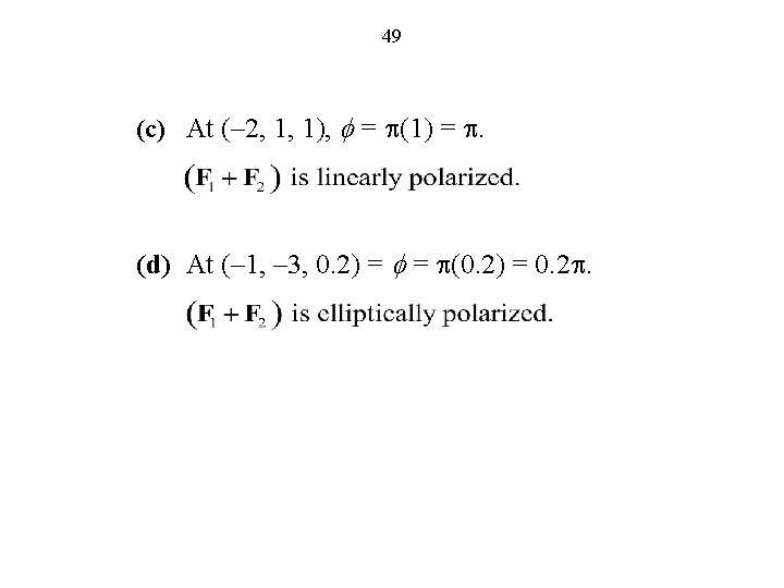
48 D 3. 17 F 1 and F 2 are equal in amplitude (= F 0) and differ in direction by 90˚. The phase difference (say f) depends on z in the manner – 2 pz – (– 3 pz) = pz. (a) At (3, 4, 0), f = p(0) = 0. (b) At (3, – 2, 0. 5), f = p(0. 5) = 0. 5 p.

50 Power Flow and Energy Storage (FEME, Sec. 4. 6; EEE 6 E, Sec. 3. 7)

Power Flow and Energy Storage Ñ (E x H) = H (Ñ x E) – E (Ñ x H) A Vector Identity D B ¶ ¶ – H× Ñ × (Ex H) = –E × J – E × ¶t ¶t For 2ö 2ö 1 1 ¶ ¶ æ æ -E × J 0 = s E + è e E ø + è m H ø + Ñ× (E x H) ¶t 2 2 Define P = E x H Poynting Vector 41

Poynting’s Theorem Power dissipation density Source power density Magnetic stored energy density Electric stored energy density 42

Interpretation of Poynting’s Theorem says that the power delivered to the volume V by the current source J 0 is accounted for by the power dissipated in the volume due to the conduction current in the medium, plus the time rates of increase of the energies stored in the electric and magnetic fields, plus another term, which we must interpret as the power carried by the electromagnetic field out of the volume V, for conservation of energy to be satisfied. It then follows that the Poynting vector P has the meaning of power flow density vector associated with the electromagnetic field. We note that the units of E x H are volts per meter times amperes per meter, or watts per square meter (W/m 2) and do indeed represent power density. 43

The End