From Vertices to Fragments Software College Shandong University

From Vertices to Fragments Software College, Shandong University Instructor: Zhou Yuanfeng E-mail: yuanfeng. zhou@gmail. com

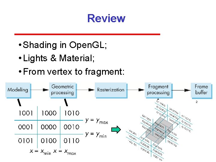
Review • Shading in Open. GL; • Lights & Material; • From vertex to fragment: 2 • Cohen Sutherland Black box Projection Fragments Clipping Shading Surface hidden Texture Transparency

Objectives • Geometric Processing: Cyrus Beck clipping algorithm Liang Barsky clipping algorithm • Introduce clipping algorithm for polygons • Rasterization: DDA & Bresenham 3

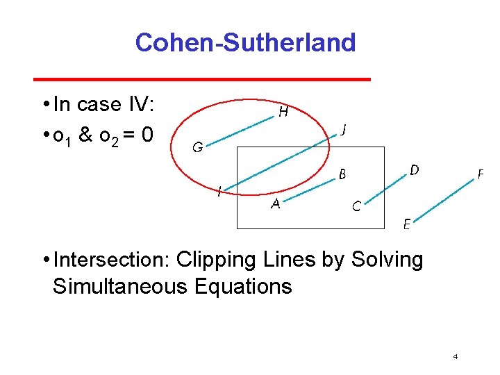
Cohen-Sutherland • In case IV: • o 1 & o 2 = 0 • Intersection: Clipping Lines by Solving Simultaneous Equations 4

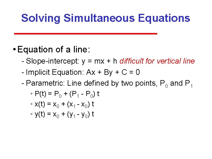
Solving Simultaneous Equations • Equation of a line: Slope intercept: y = mx + h difficult for vertical line Implicit Equation: Ax + By + C = 0 Parametric: Line defined by two points, P 0 and P 1 • P(t) = P 0 + (P 1 P 0) t • x(t) = x 0 + (x 1 x 0) t • y(t) = x 0 + (y 1 y 0) t

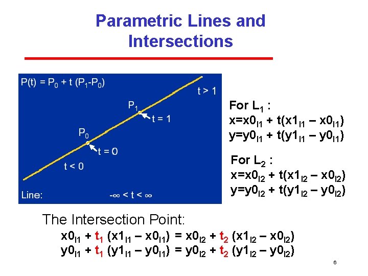
Parametric Lines and Intersections For L 1 : x=x 0 l 1 + t(x 1 l 1 – x 0 l 1) y=y 0 l 1 + t(y 1 l 1 – y 0 l 1) For L 2 : x=x 0 l 2 + t(x 1 l 2 – x 0 l 2) y=y 0 l 2 + t(y 1 l 2 – y 0 l 2) The Intersection Point: x 0 l 1 + t 1 (x 1 l 1 – x 0 l 1) = x 0 l 2 + t 2 (x 1 l 2 – x 0 l 2) y 0 l 1 + t 1 (y 1 l 1 – y 0 l 1) = y 0 l 2 + t 2 (y 1 l 2 – y 0 l 2) 6

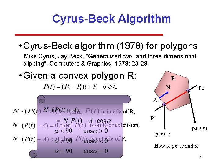
Cyrus-Beck Algorithm • Cyrus Beck algorithm (1978) for polygons Mike Cyrus, Jay Beck. "Generalized two and three dimensional clipping". Computers & Graphics, 1978: 23 28. • Given a convex polygon R: R 0≤t≤ 1 N P 2 A , then is inside of R; P 1 , then is on R or extension; is outside of R. para ts para te How to get ts and te 7

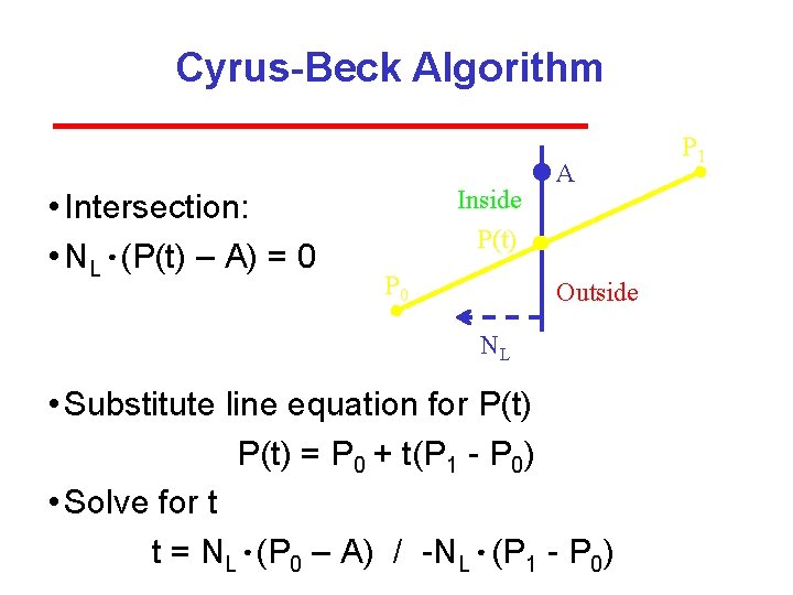
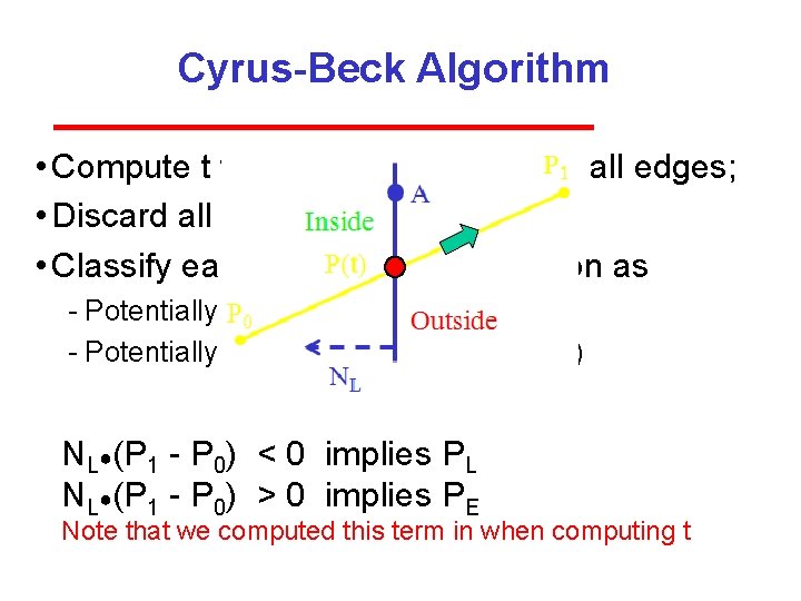
Cyrus-Beck Algorithm • Intersection: • NL ● (P(t) – A) = 0 Inside P(t) P 0 A Outside NL • Substitute line equation for P(t) = P 0 + t(P 1 P 0) • Solve for t t = NL ● (P 0 – A) / NL ● (P 1 P 0) P 1

Cyrus-Beck Algorithm • Compute t for line intersection with all edges; • Discard all (t < 0) and (t > 1); • Classify each remaining intersection as Potentially Entering Point (PE) Potentially Leaving Point (PL) (How? ) NL●(P 1 P 0) < 0 implies PL NL●(P 1 P 0) > 0 implies PE Note that we computed this term in when computing t

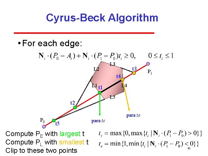
Cyrus-Beck Algorithm • For each edge: L 2 L 3 t 4 L 1 t 5 Compute PE with largest t Compute PL with smallest t Clip to these two points L 4 L 5 t 2 P 0 P 1 para ts para te 10

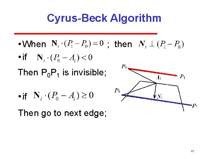
Cyrus-Beck Algorithm • When • if ; then Then P 0 P 1 is invisible; • if Then go to next edge; 11

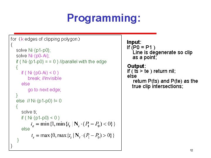
Programming: for（k edges of clipping polygon） { solve Ni·(p 1 p 0); solve Ni·(p 0 Ai); if ( Ni·(p 1 p 0) = = 0 ) //parallel with the edge { if ( Ni·(p 0 Ai) < 0 ) break; //invisible else go to next edge; } else // Ni·(p 1 p 0) != 0 { solve ti; if ( Ni·(p 1 p 0) < 0 ) Input: If (P 0 = P 1 ) Line is degenerate so clip as a point; Output: if ( ts > te ) return nil; else return P(ts) and P(te) as the true clip intersections; else } } 12

Liang-Barsky Algorithm (1984) The ONLY algorithm named for Chinese people in Computer Graphics course books Liang, Y. D. , and Barsky, B. , "A New Concept and Method for Line Clipping", ACM Transactions on Graphics, 3(1): 113 22, January 1984.

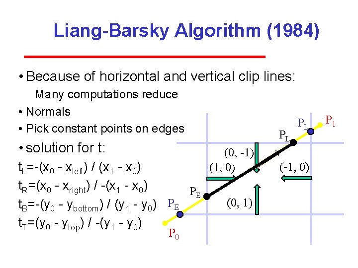
Liang-Barsky Algorithm (1984) • Because of horizontal and vertical clip lines: Many computations reduce • Normals • Pick constant points on edges • solution for t: t. L= (x 0 xleft) / (x 1 x 0) t. R=(x 0 xright) / (x 1 x 0) PE t. B= (y 0 ybottom) / (y 1 y 0) PE t. T=(y 0 ytop) / (y 1 y 0) P 0 PL (0, -1) (1, 0) (0, 1) PL (-1, 0) P 1

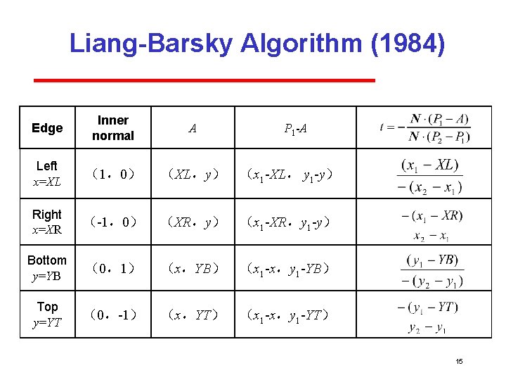
Liang-Barsky Algorithm (1984) Edge Inner normal A Left x=XL （1，0） （XL，y） （x 1 -XL， y 1 -y） Right x=XR （-1，0） （XR，y） （x 1 -XR，y 1 -y） Bottom y=YB （0，1） （x，YB） （x 1 -x，y 1 -YB） Top y=YT （0，-1） （x，YT） （x 1 -x，y 1 -YT） P 1 -A 15

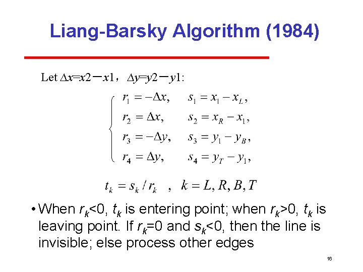
Liang-Barsky Algorithm (1984) Let ∆x=x 2－x 1，∆y=y 2－y 1: • When rk<0, tk is entering point; when rk>0, tk is leaving point. If rk=0 and sk<0, then the line is invisible; else process other edges 16

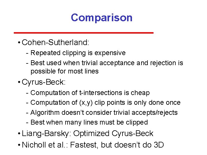
Comparison • Cohen Sutherland: Repeated clipping is expensive Best used when trivial acceptance and rejection is possible for most lines • Cyrus Beck: Computation of t intersections is cheap Computation of (x, y) clip points is only done once Algorithm doesn’t consider trivial accepts/rejects Best when many lines must be clipped • Liang Barsky: Optimized Cyrus Beck • Nicholl et al. : Fastest, but doesn’t do 3 D

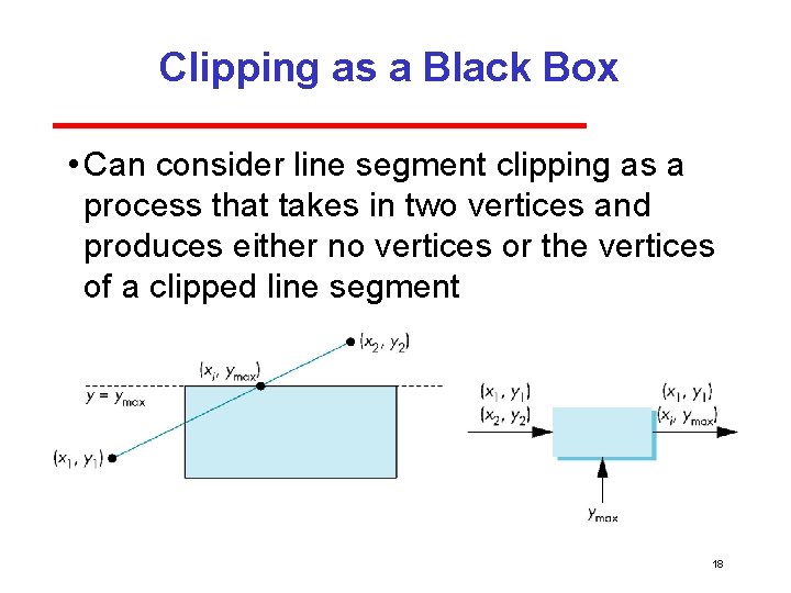
Clipping as a Black Box • Can consider line segment clipping as a process that takes in two vertices and produces either no vertices or the vertices of a clipped line segment 18

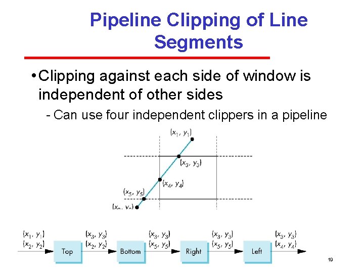
Pipeline Clipping of Line Segments • Clipping against each side of window is independent of other sides Can use four independent clippers in a pipeline 19

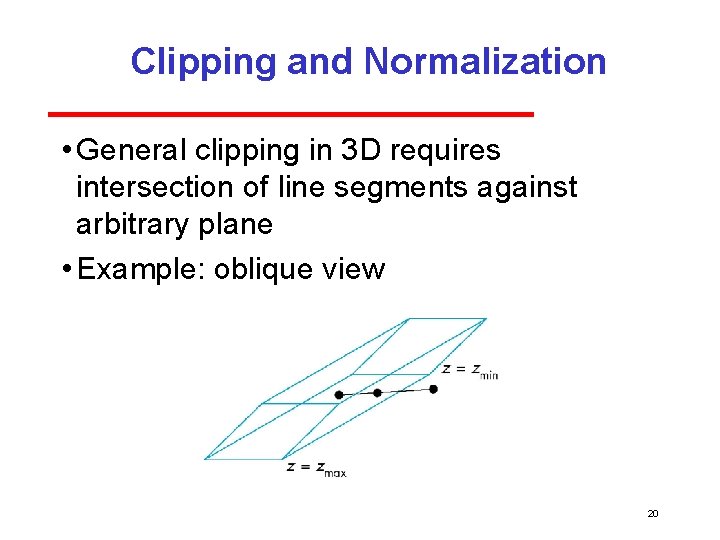
Clipping and Normalization • General clipping in 3 D requires intersection of line segments against arbitrary plane • Example: oblique view 20

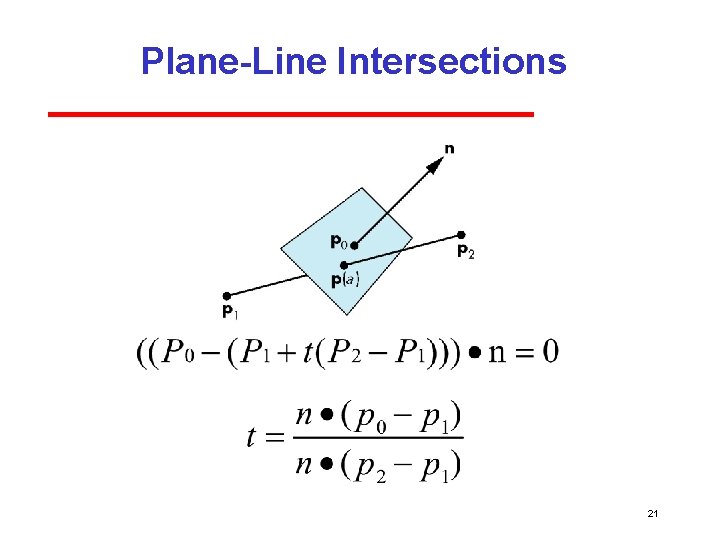
Plane-Line Intersections 21

Point-to-Plane Test • Dot product is relatively expensive 3 multiplies 5 additions 1 comparison (to 0, in this case) • Think about how you might optimize or special case this?

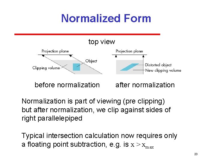
Normalized Form top view before normalization after normalization Normalization is part of viewing (pre clipping) but after normalization, we clip against sides of right parallelepiped Typical intersection calculation now requires only a floating point subtraction, e. g. is x > xmax 23

Clipping Polygons • Clipping polygons is more complex than clipping the individual lines Input: polygon Output: polygon, or nothing

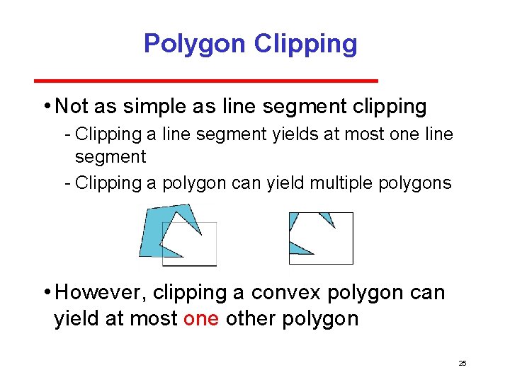
Polygon Clipping • Not as simple as line segment clipping Clipping a line segment yields at most one line segment Clipping a polygon can yield multiple polygons • However, clipping a convex polygon can yield at most one other polygon 25

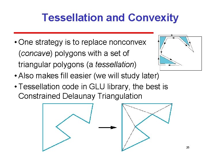
Tessellation and Convexity • One strategy is to replace nonconvex (concave) polygons with a set of triangular polygons (a tessellation) • Also makes fill easier (we will study later) • Tessellation code in GLU library, the best is Constrained Delaunay Triangulation 26

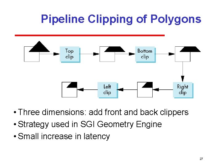
Pipeline Clipping of Polygons • Three dimensions: add front and back clippers • Strategy used in SGI Geometry Engine • Small increase in latency 27

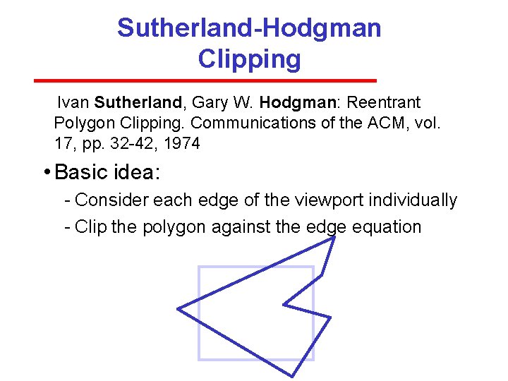
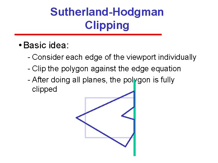
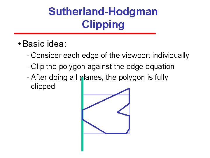
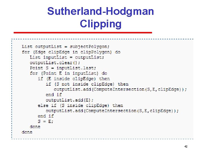
Sutherland-Hodgman Clipping Ivan Sutherland, Gary W. Hodgman: Reentrant Polygon Clipping. Communications of the ACM, vol. 17, pp. 32 42, 1974 • Basic idea: Consider each edge of the viewport individually Clip the polygon against the edge equation

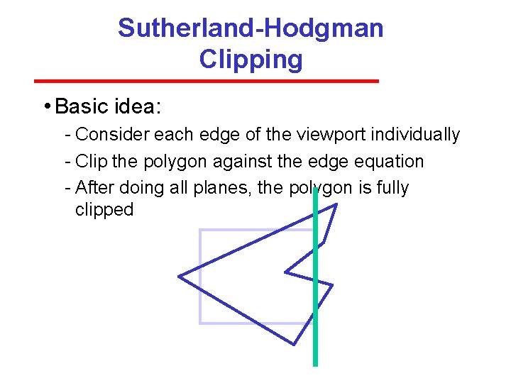
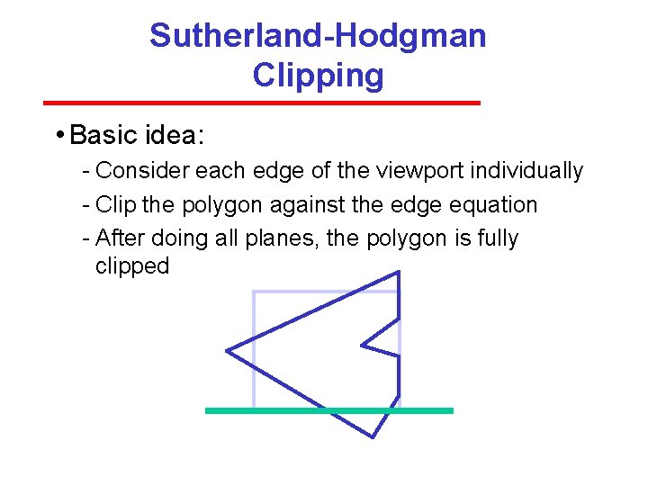
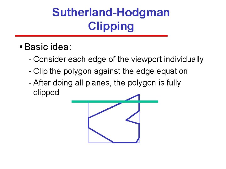
Sutherland-Hodgman Clipping • Basic idea: Consider each edge of the viewport individually Clip the polygon against the edge equation After doing all planes, the polygon is fully clipped

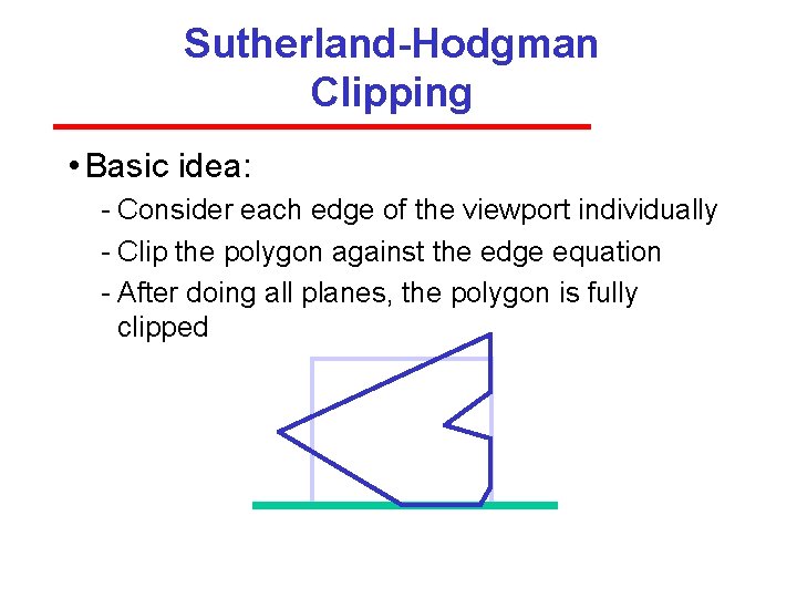
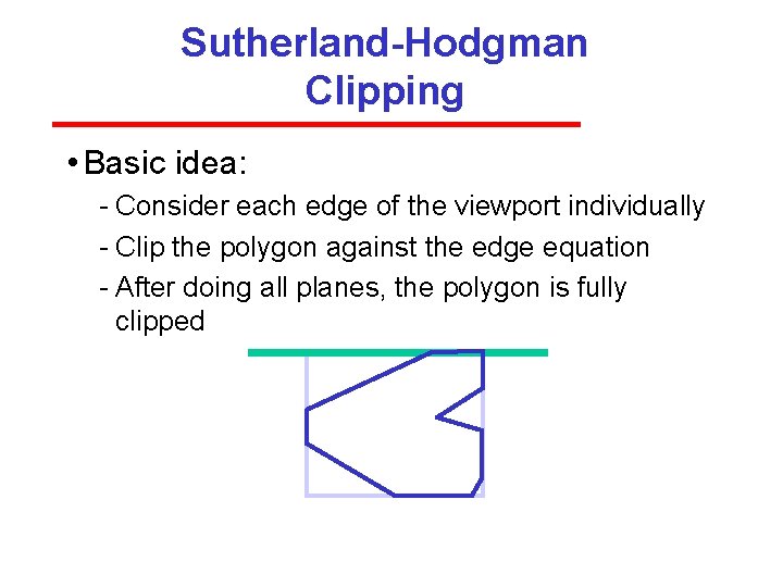
Sutherland-Hodgman Clipping • Basic idea: Consider each edge of the viewport individually Clip the polygon against the edge equation After doing all planes, the polygon is fully clipped

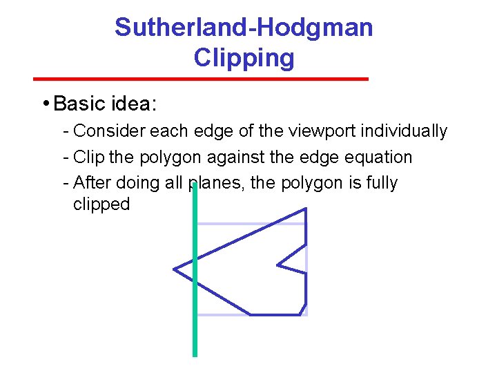
Sutherland-Hodgman Clipping • Basic idea: Consider each edge of the viewport individually Clip the polygon against the edge equation After doing all planes, the polygon is fully clipped

Sutherland-Hodgman Clipping • Basic idea: Consider each edge of the viewport individually Clip the polygon against the edge equation After doing all planes, the polygon is fully clipped

Sutherland-Hodgman Clipping • Basic idea: Consider each edge of the viewport individually Clip the polygon against the edge equation After doing all planes, the polygon is fully clipped

Sutherland-Hodgman Clipping • Basic idea: Consider each edge of the viewport individually Clip the polygon against the edge equation After doing all planes, the polygon is fully clipped

Sutherland-Hodgman Clipping • Basic idea: Consider each edge of the viewport individually Clip the polygon against the edge equation After doing all planes, the polygon is fully clipped

Sutherland-Hodgman Clipping • Basic idea: Consider each edge of the viewport individually Clip the polygon against the edge equation After doing all planes, the polygon is fully clipped

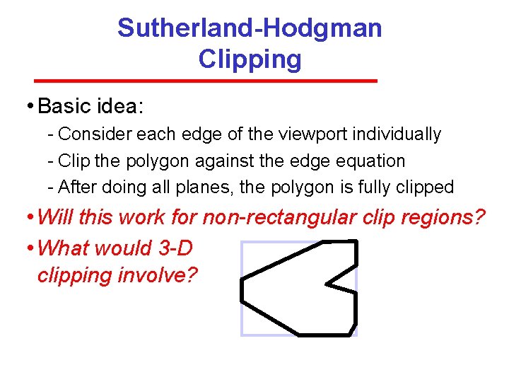
Sutherland-Hodgman Clipping • Basic idea: Consider each edge of the viewport individually Clip the polygon against the edge equation After doing all planes, the polygon is fully clipped • Will this work for non-rectangular clip regions? • What would 3 -D clipping involve?

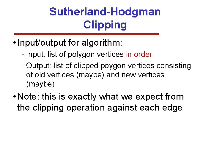
Sutherland-Hodgman Clipping • Input/output for algorithm: Input: list of polygon vertices in order Output: list of clipped poygon vertices consisting of old vertices (maybe) and new vertices (maybe) • Note: this is exactly what we expect from the clipping operation against each edge

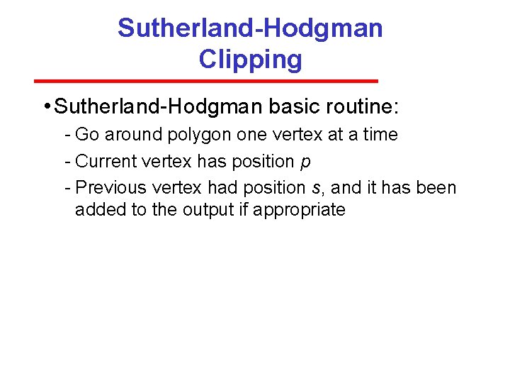
Sutherland-Hodgman Clipping • Sutherland Hodgman basic routine: Go around polygon one vertex at a time Current vertex has position p Previous vertex had position s, and it has been added to the output if appropriate

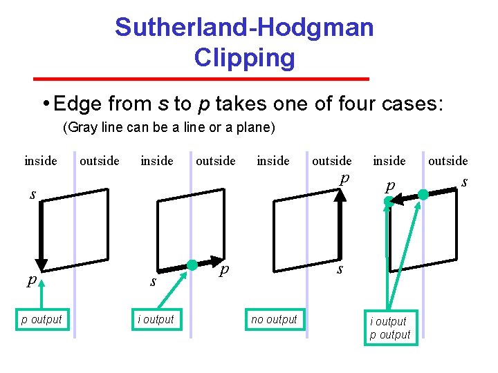
Sutherland-Hodgman Clipping • Edge from s to p takes one of four cases: (Gray line can be a line or a plane) inside outside inside s p p output s i output p outside p inside p s no output i output p output outside s

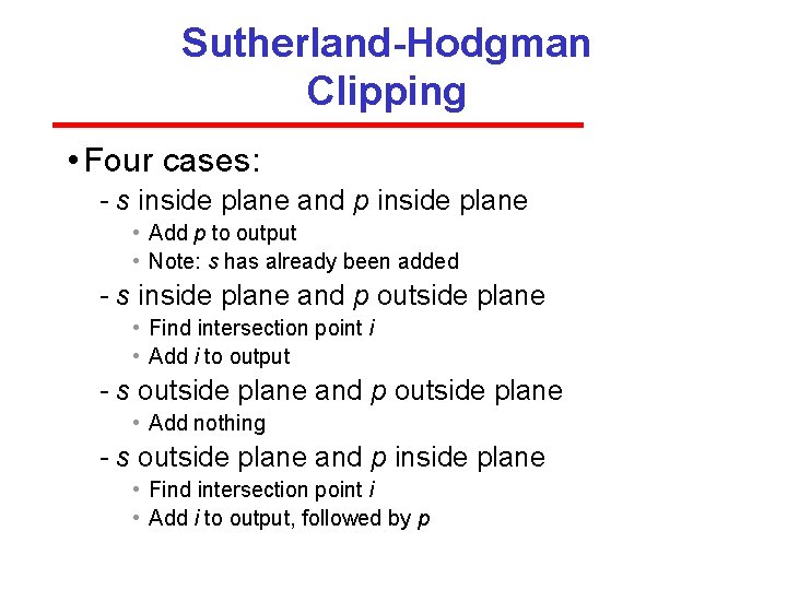
Sutherland-Hodgman Clipping • Four cases: s inside plane and p inside plane • Add p to output • Note: s has already been added s inside plane and p outside plane • Find intersection point i • Add i to output s outside plane and p outside plane • Add nothing s outside plane and p inside plane • Find intersection point i • Add i to output, followed by p

Sutherland-Hodgman Clipping 42

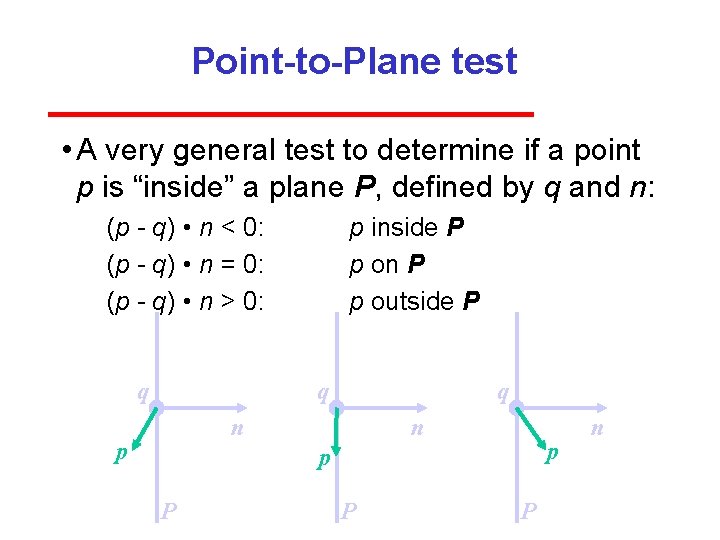
Point-to-Plane test • A very general test to determine if a point p is “inside” a plane P, defined by q and n: (p q) • n < 0: (p q) • n = 0: (p q) • n > 0: q p inside P p on P p outside P q q n p p P P P n

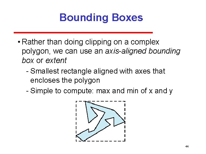
Bounding Boxes • Rather than doing clipping on a complex polygon, we can use an axis-aligned bounding box or extent Smallest rectangle aligned with axes that encloses the polygon Simple to compute: max and min of x and y 44

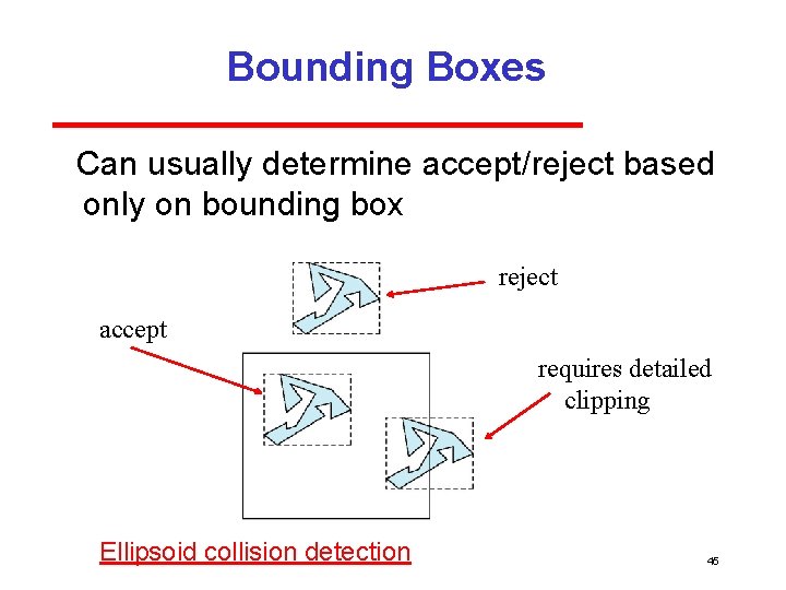
Bounding Boxes Can usually determine accept/reject based only on bounding box reject accept requires detailed clipping Ellipsoid collision detection 45

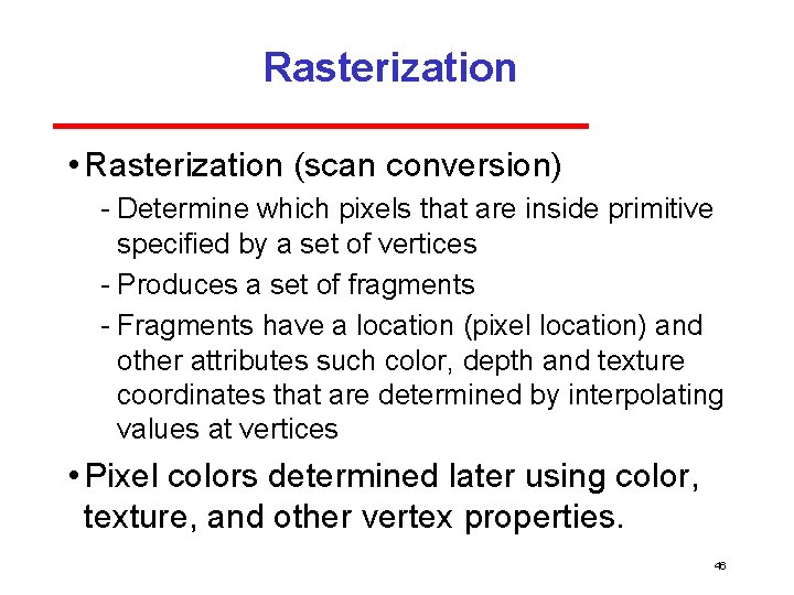
Rasterization • Rasterization (scan conversion) Determine which pixels that are inside primitive specified by a set of vertices Produces a set of fragments Fragments have a location (pixel location) and other attributes such color, depth and texture coordinates that are determined by interpolating values at vertices • Pixel colors determined later using color, texture, and other vertex properties. 46

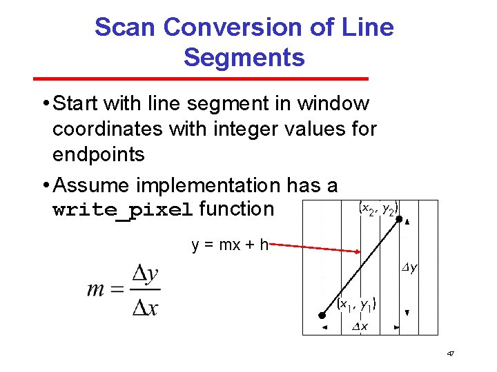
Scan Conversion of Line Segments • Start with line segment in window coordinates with integer values for endpoints • Assume implementation has a write_pixel function y = mx + h 47

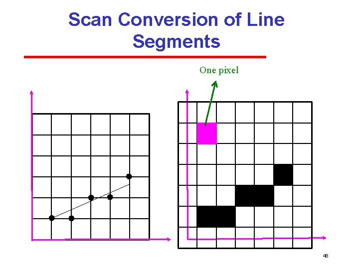
Scan Conversion of Line Segments One pixel 48

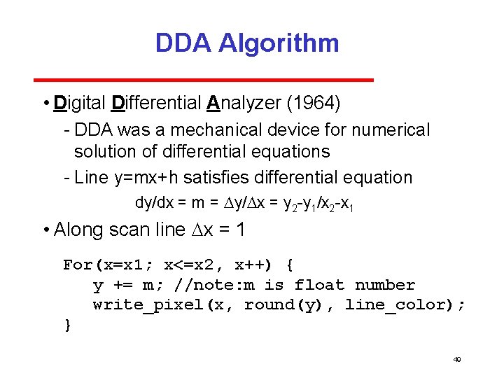
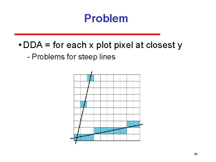
DDA Algorithm • Digital Differential Analyzer (1964) DDA was a mechanical device for numerical solution of differential equations Line y=mx+h satisfies differential equation dy/dx = m = y/ x = y 2 y 1/x 2 x 1 • Along scan line x = 1 For(x=x 1; x<=x 2, x++) { y += m; //note: m is float number write_pixel(x, round(y), line_color); } 49

Problem • DDA = for each x plot pixel at closest y Problems for steep lines 50

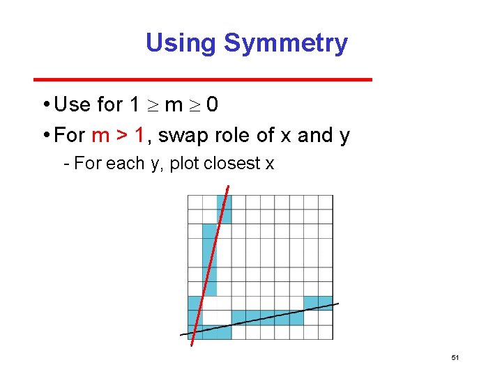
Using Symmetry • Use for 1 m 0 • For m > 1, swap role of x and y For each y, plot closest x 51

Bresenham’s Algorithm • DDA requires one floating point addition per step • We can eliminate all fp through Bresenham’s algorithm • Consider only 1 m 0 Other cases by symmetry • Assume pixel centers are at half integers (Open. GL has this definition) Bresenham, J. E. (1 January 1965). "Algorithm for computer control of a digital plotter". IBM Systems Journal 4(1): 25– 30. 52

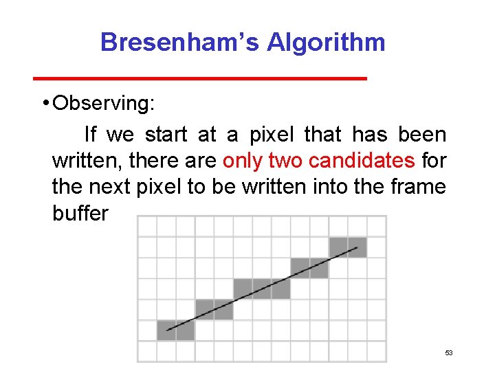
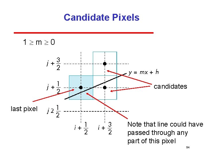
Bresenham’s Algorithm • Observing: If we start at a pixel that has been written, there are only two candidates for the next pixel to be written into the frame buffer 53

Candidate Pixels 1 m 0 candidates last pixel Note that line could have passed through any part of this pixel 54

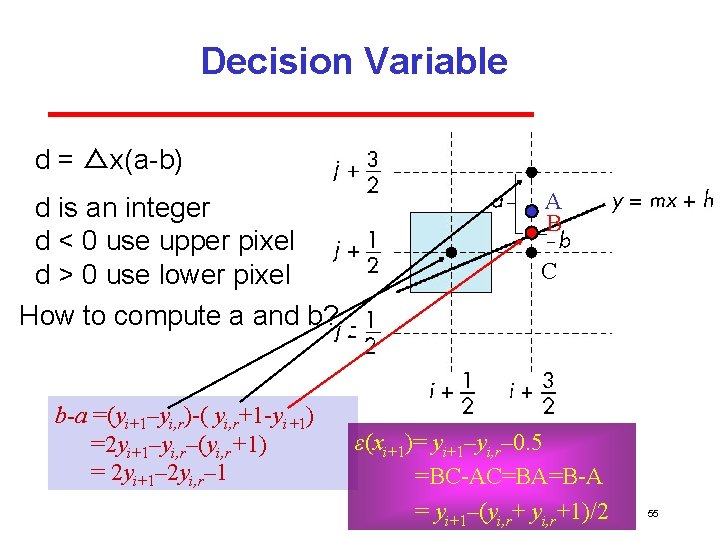
Decision Variable d = △x(a b) d is an integer d < 0 use upper pixel d > 0 use lower pixel How to compute a and b? b-a =(yi+1–yi, r)-( yi, r+1 -yi+1) =2 yi+1–yi, r–(yi, r+1) = 2 yi+1– 2 yi, r– 1 A B C - ε(xi+1)= yi+1–yi, r– 0. 5 =BC-AC=BA=B-A = yi+1–(yi, r+1)/2 55

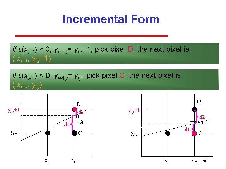
Incremental Form if ε(xi+1) ≥ 0, yi+1, r= yi, r+1, pick pixel D, the next pixel is ( xi+1, yi, r+1) if ε(xi+1) < 0, yi+1, r= yi, r, pick pixel C, the next pixel is ( xi+1, yi, r) yi, r+1 d 1 yi, r xi D D d 2 B A yi, r+1 C yi, r xi+1 d 2 A d 1 xi C xi+1 56

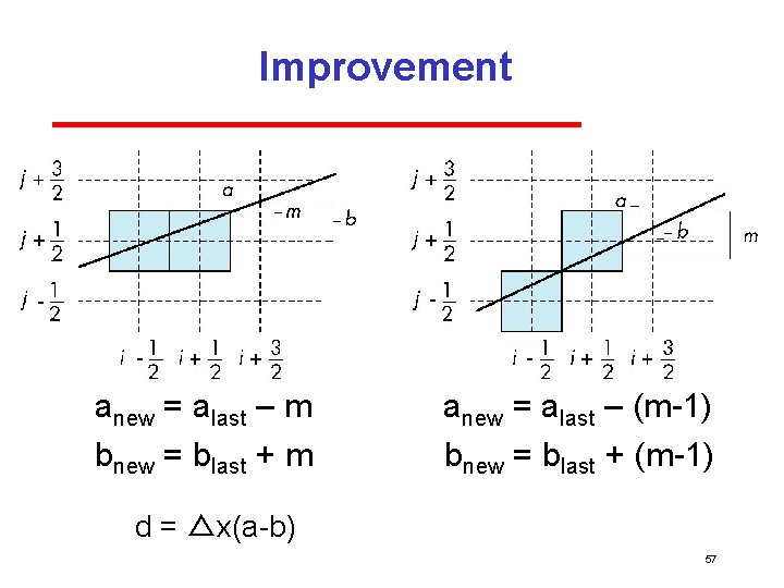
Improvement - - anew = alast – m bnew = blast + m - anew = alast – (m 1) bnew = blast + (m 1) d = △x(a b) 57

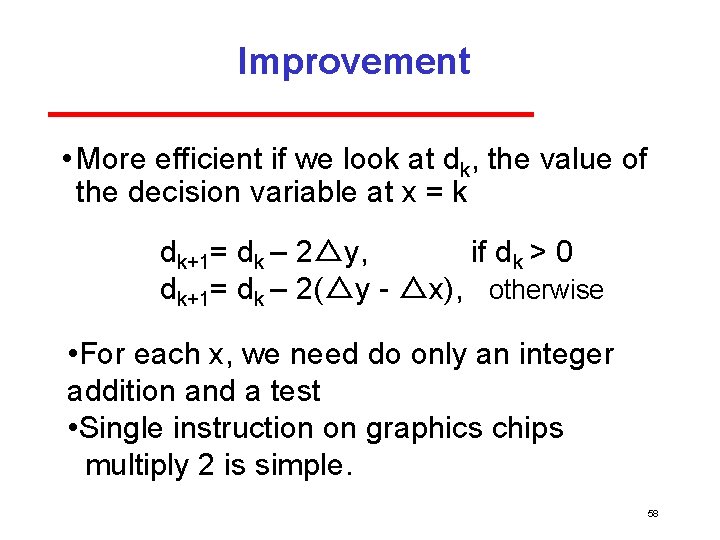
Improvement • More efficient if we look at dk, the value of the decision variable at x = k dk+1= dk – 2△y, if dk > 0 dk+1= dk – 2(△y △x), otherwise • For each x, we need do only an integer addition and a test • Single instruction on graphics chips multiply 2 is simple. 58

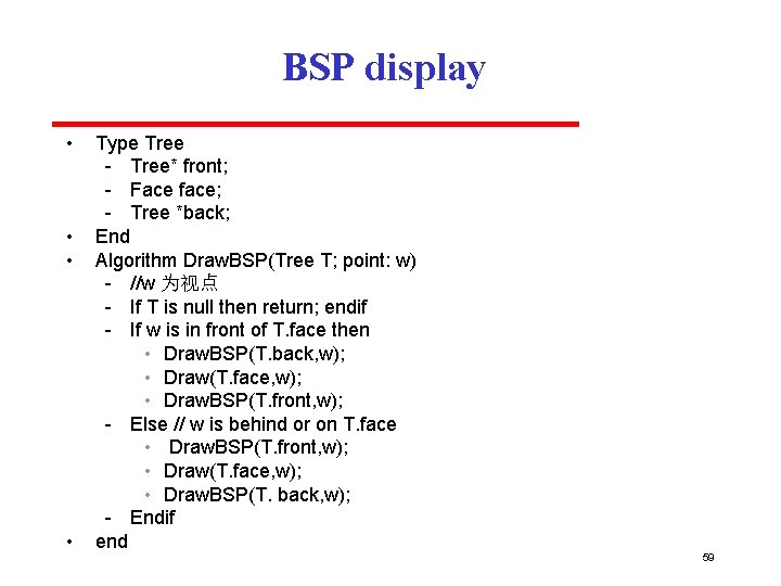
BSP display • • Type Tree* front; Face face; Tree *back; End Algorithm Draw. BSP(Tree T; point: w) //w 为视点 If T is null then return; endif If w is in front of T. face then • Draw. BSP(T. back, w); • Draw(T. face, w); • Draw. BSP(T. front, w); Else // w is behind or on T. face • Draw. BSP(T. front, w); • Draw(T. face, w); • Draw. BSP(T. back, w); Endif end 59

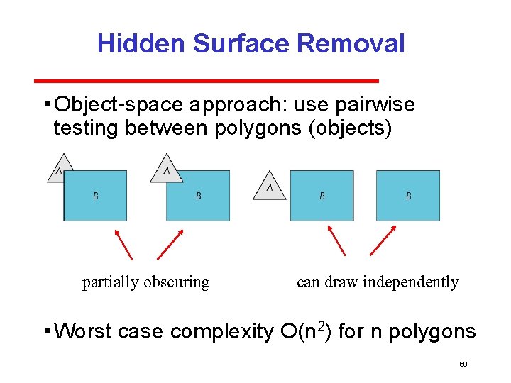
Hidden Surface Removal • Object space approach: use pairwise testing between polygons (objects) partially obscuring can draw independently • Worst case complexity O(n 2) for n polygons 60

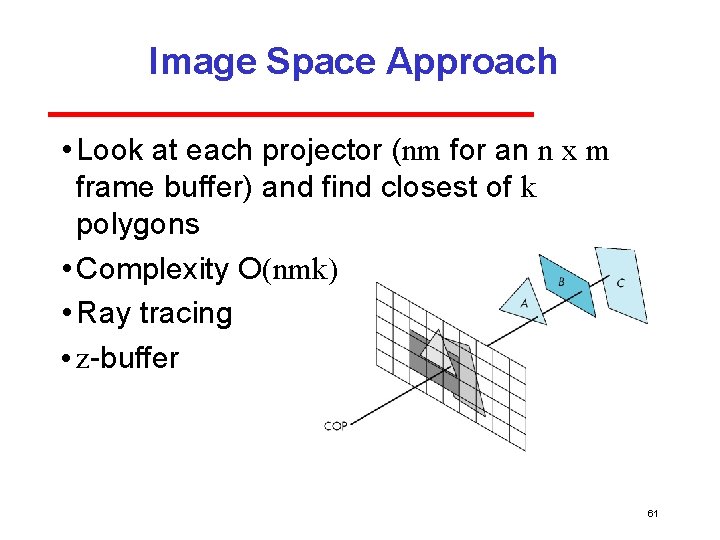
Image Space Approach • Look at each projector (nm for an n x m frame buffer) and find closest of k polygons • Complexity O(nmk) • Ray tracing • z buffer 61

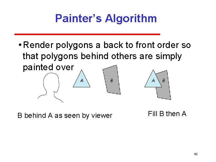
Painter’s Algorithm • Render polygons a back to front order so that polygons behind others are simply painted over B behind A as seen by viewer Fill B then A 62

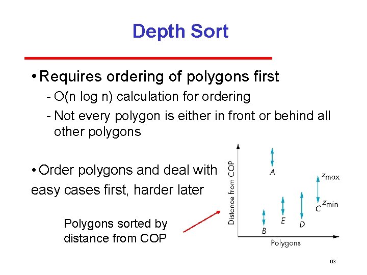
Depth Sort • Requires ordering of polygons first O(n log n) calculation for ordering Not every polygon is either in front or behind all other polygons • Order polygons and deal with easy cases first, harder later Polygons sorted by distance from COP 63

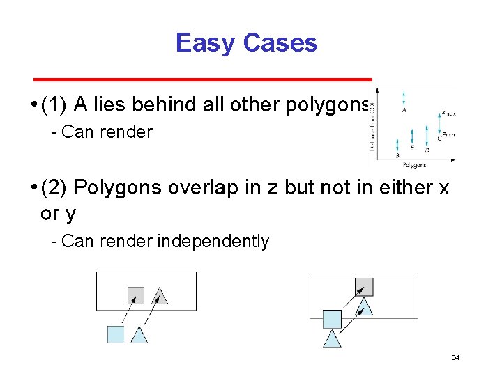
Easy Cases • (1) A lies behind all other polygons Can render • (2) Polygons overlap in z but not in either x or y Can render independently 64

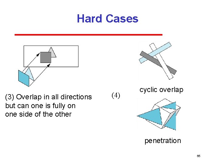
Hard Cases (3) Overlap in all directions but can one is fully on one side of the other (4) cyclic overlap penetration 65

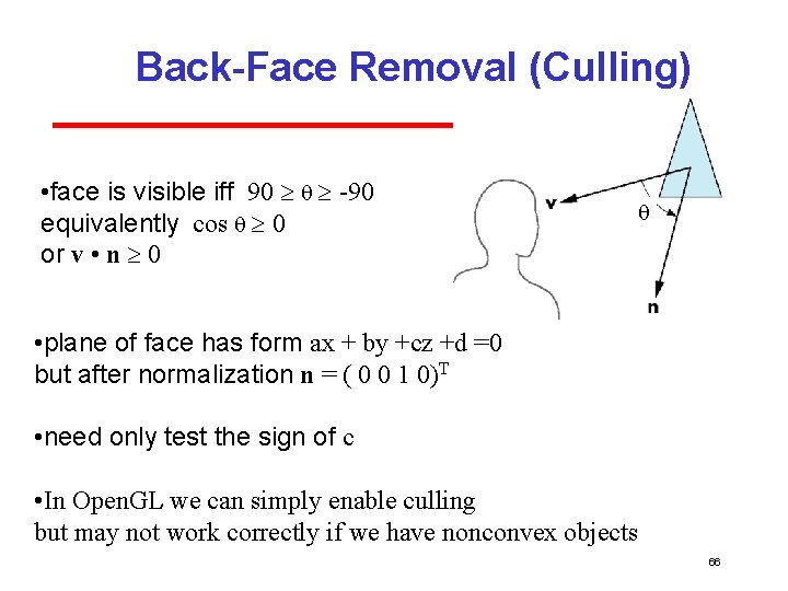
Back-Face Removal (Culling) • face is visible iff 90 -90 equivalently cos 0 or v • n 0 • plane of face has form ax + by +cz +d =0 but after normalization n = ( 0 0 1 0)T • need only test the sign of c • In Open. GL we can simply enable culling but may not work correctly if we have nonconvex objects 66

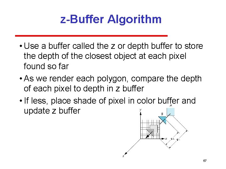
z-Buffer Algorithm • Use a buffer called the z or depth buffer to store the depth of the closest object at each pixel found so far • As we render each polygon, compare the depth of each pixel to depth in z buffer • If less, place shade of pixel in color buffer and update z buffer 67

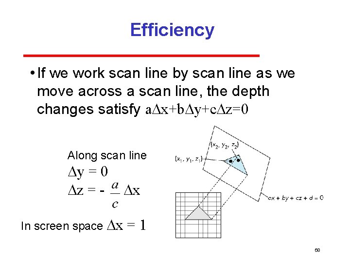
Efficiency • If we work scan line by scan line as we move across a scan line, the depth changes satisfy a x+b y+c z=0 Along scan line y = 0 z = - In screen space x x =1 68

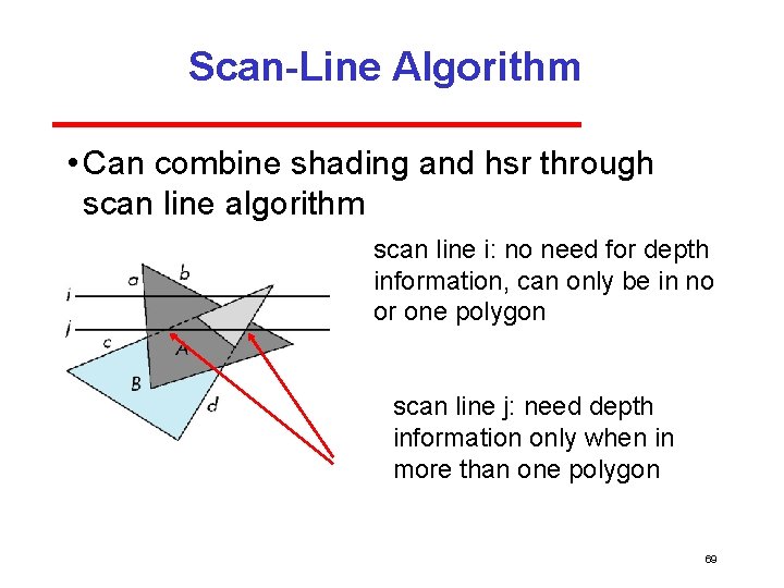
Scan-Line Algorithm • Can combine shading and hsr through scan line algorithm scan line i: no need for depth information, can only be in no or one polygon scan line j: need depth information only when in more than one polygon 69

Implementation • Need a data structure to store Flag for each polygon (inside/outside) Incremental structure for scan lines that stores which edges are encountered Parameters for planes 70

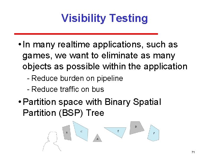
Visibility Testing • In many realtime applications, such as games, we want to eliminate as many objects as possible within the application Reduce burden on pipeline Reduce traffic on bus • Partition space with Binary Spatial Partition (BSP) Tree 71

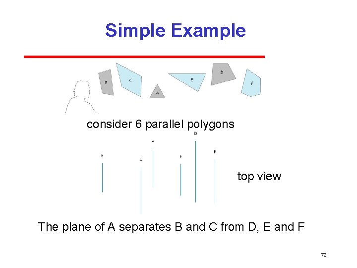
Simple Example consider 6 parallel polygons top view The plane of A separates B and C from D, E and F 72

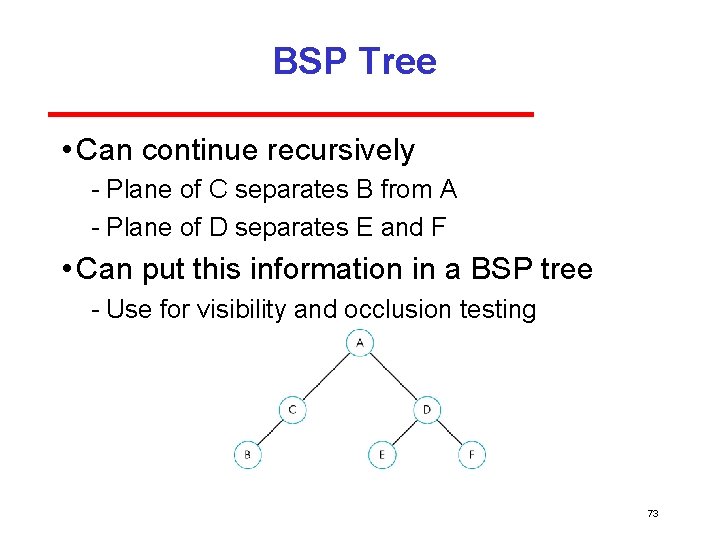
BSP Tree • Can continue recursively Plane of C separates B from A Plane of D separates E and F • Can put this information in a BSP tree Use for visibility and occlusion testing 73

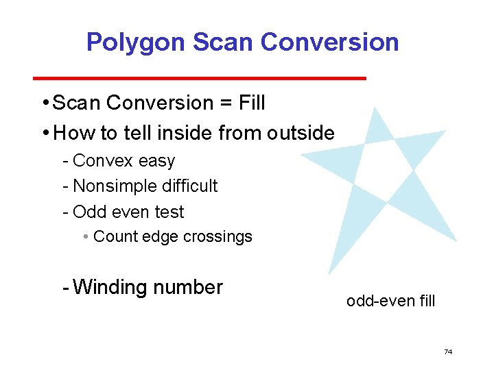
Polygon Scan Conversion • Scan Conversion = Fill • How to tell inside from outside Convex easy Nonsimple difficult Odd even test • Count edge crossings Winding number odd even fill 74

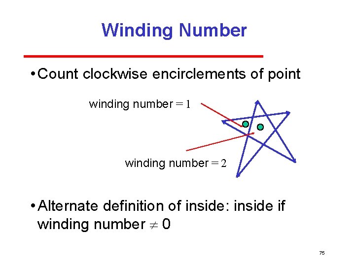
Winding Number • Count clockwise encirclements of point winding number = 1 winding number = 2 • Alternate definition of inside: inside if winding number 0 75

Filling in the Frame Buffer • Fill at end of pipeline Convex Polygons only Nonconvex polygons assumed to have been tessellated Shades (colors) have been computed for vertices (Gouraud shading) Combine with z buffer algorithm • March across scan lines interpolating shades • Incremental work small 76

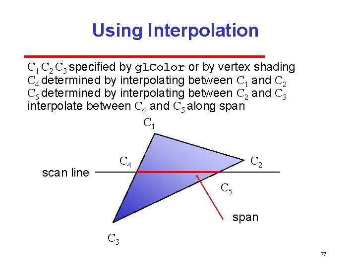
Using Interpolation C 1 C 2 C 3 specified by gl. Color or by vertex shading C 4 determined by interpolating between C 1 and C 2 C 5 determined by interpolating between C 2 and C 3 interpolate between C 4 and C 5 along span C 1 C 4 scan line C 2 C 5 span C 3 77

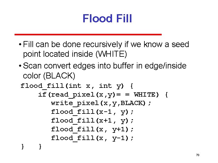
Flood Fill • Fill can be done recursively if we know a seed point located inside (WHITE) • Scan convert edges into buffer in edge/inside color (BLACK) flood_fill(int x, int y) { if(read_pixel(x, y)= = WHITE) { write_pixel(x, y, BLACK); flood_fill(x-1, y); flood_fill(x+1, y); flood_fill(x, y+1); flood_fill(x, y-1); } } 78

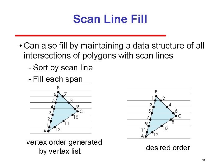
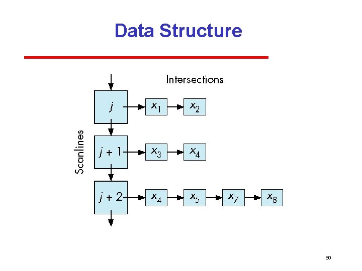
Scan Line Fill • Can also fill by maintaining a data structure of all intersections of polygons with scan lines Sort by scan line Fill each span vertex order generated by vertex list desired order 79

Data Structure 80

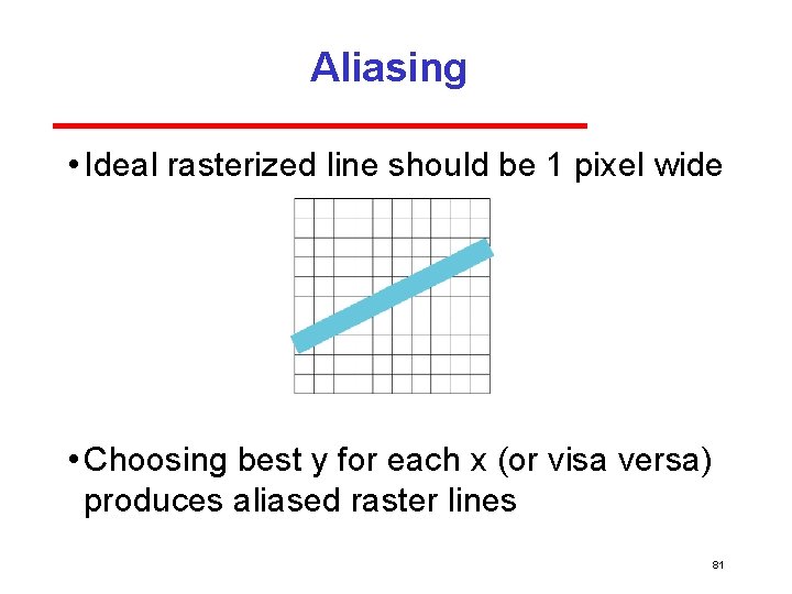
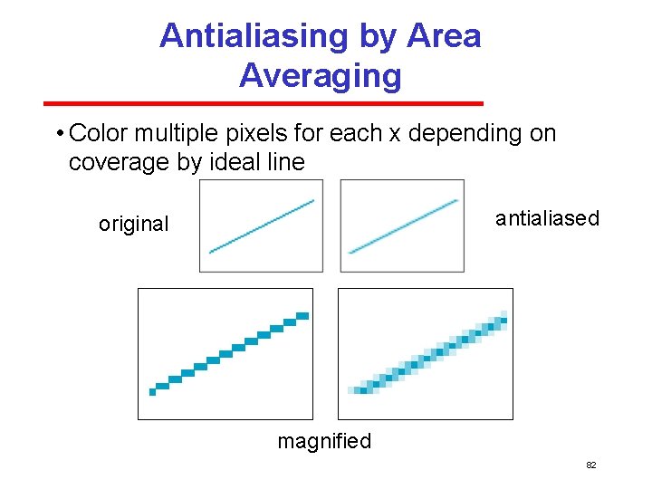
Aliasing • Ideal rasterized line should be 1 pixel wide • Choosing best y for each x (or visa versa) produces aliased raster lines 81

Antialiasing by Area Averaging • Color multiple pixels for each x depending on coverage by ideal line antialiased original magnified 82

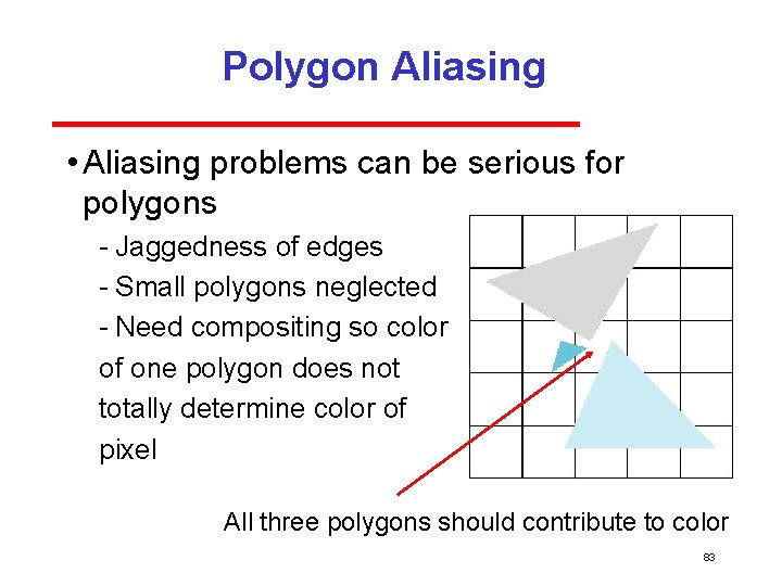
Polygon Aliasing • Aliasing problems can be serious for polygons Jaggedness of edges Small polygons neglected Need compositing so color of one polygon does not totally determine color of pixel All three polygons should contribute to color 83