From Vertices to Fragments II Software College Shandong

From Vertices to Fragments II Software College, Shandong University Instructor: Zhou Yuanfeng E-mail: yuanfeng. zhou@gmail. com

Review • Cyrus Beck clipping algorithm; • Liang Barsky clipping algorithm; • Sutherland Hodgman polygon clipping; • DDA line algorithm; • Bresenham’s line algorithm;

Objectives • Rasterization: Polygon scan conversion algorithm; • Hidden surface removal • Aliasing 3

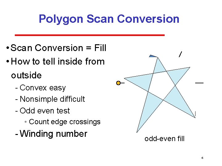
Polygon Scan Conversion • Scan Conversion = Fill • How to tell inside from outside Convex easy Nonsimple difficult Odd even test • Count edge crossings Winding number odd even fill 4

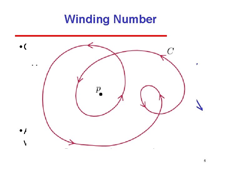
Winding Number • Count clockwise encirclements of point winding number = 1 winding number = 2 • Alternate definition of inside: inside if winding number 0 5

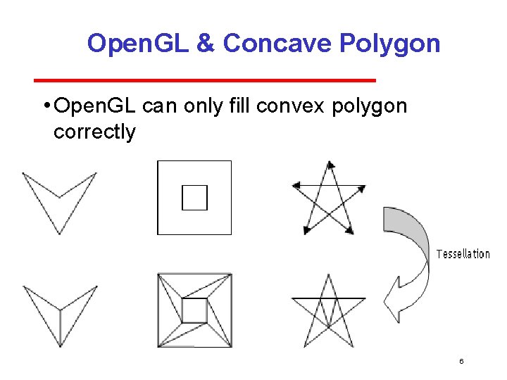
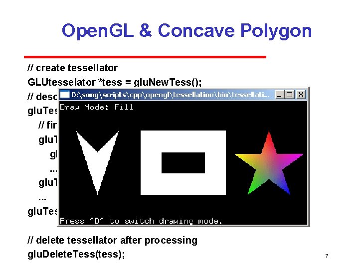
Open. GL & Concave Polygon • Open. GL can only fill convex polygon correctly 6

Open. GL & Concave Polygon // create tessellator GLUtesselator *tess = glu. New. Tess(); // describe non-convex polygon glu. Tess. Begin. Polygon(tess, user_data); // first contour glu. Tess. Begin. Contour(tess); glu. Tess. Vertex(tess, coords[0], vertex_data); . . . glu. Tess. End. Contour(tess); . . . glu. Tess. End. Polygon(tess); // delete tessellator after processing glu. Delete. Tess(tess); 7

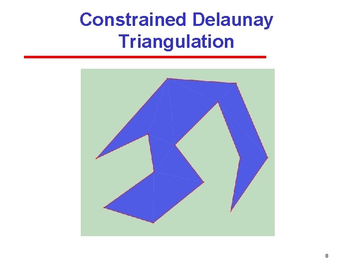
Constrained Delaunay Triangulation 8

Filling in the Frame Buffer • Fill at end of pipeline Convex Polygons only Nonconvex polygons assumed to have been tessellated Shades (colors) have been computed for vertices (Gouraud shading) Combine with z buffer algorithm • March across scan lines interpolating shades • Incremental work small 9

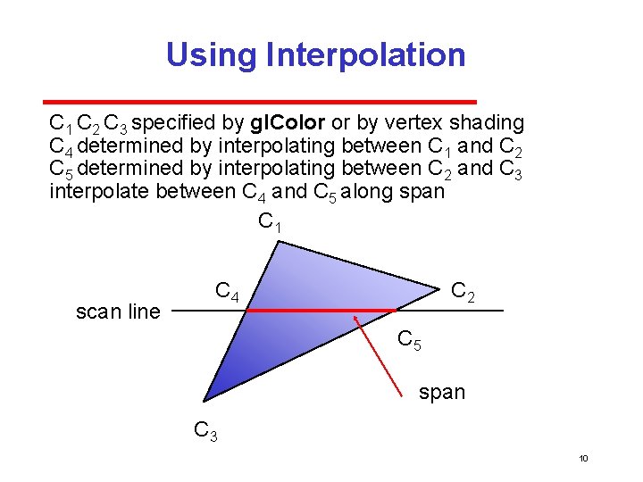
Using Interpolation C 1 C 2 C 3 specified by gl. Color or by vertex shading C 4 determined by interpolating between C 1 and C 2 C 5 determined by interpolating between C 2 and C 3 interpolate between C 4 and C 5 along span C 1 scan line C 4 C 2 C 5 span C 3 10

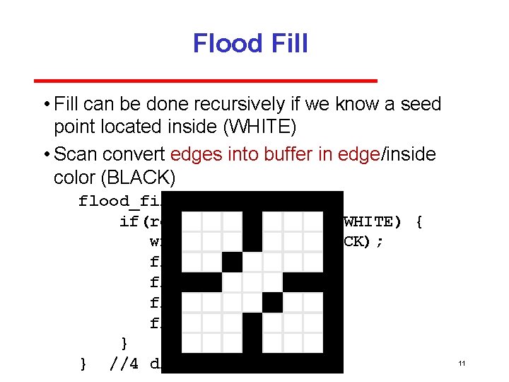
Flood Fill • Fill can be done recursively if we know a seed point located inside (WHITE) • Scan convert edges into buffer in edge/inside color (BLACK) flood_fill(int x, int y) { if(read_pixel(x, y)= = WHITE) { write_pixel(x, y, BLACK); flood_fill(x-1, y); flood_fill(x+1, y); flood_fill(x, y+1); flood_fill(x, y-1); } } //4 directions 11

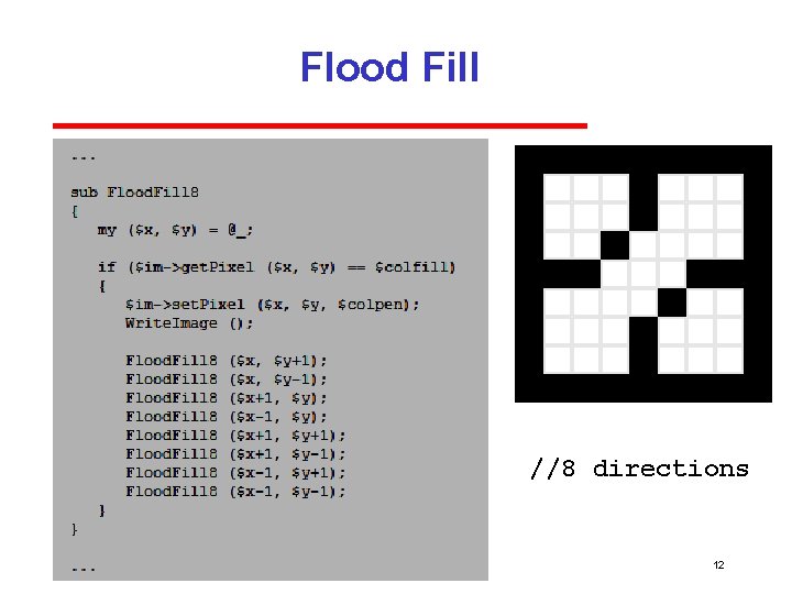
Flood Fill //8 directions 12

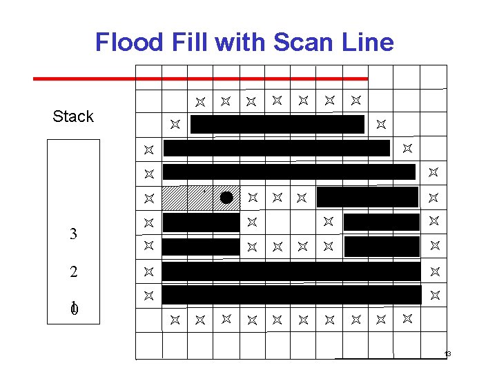
Flood Fill with Scan Line Stack 2 2 1 1 2 2 2 3 2 10 2 2 3 13

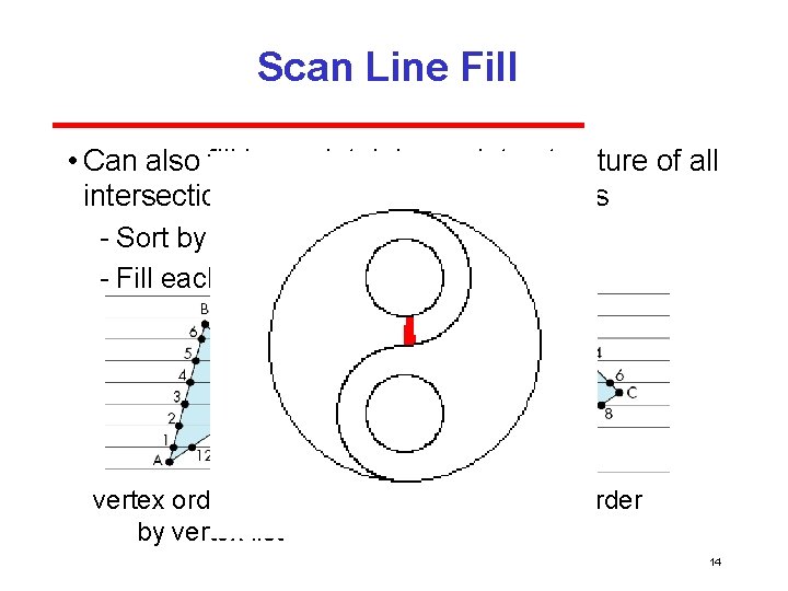
Scan Line Fill • Can also fill by maintaining a data structure of all intersections of polygons with scan lines Sort by scan line Fill each span vertex order generated by vertex list desired order 14

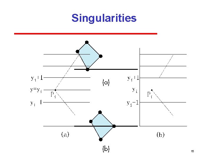
Singularities 15

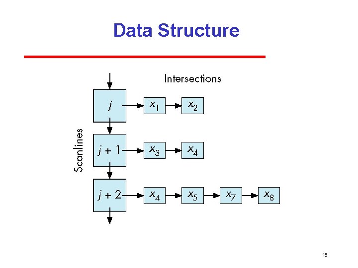
Data Structure 16

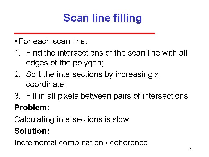
Scan line filling • For each scan line: 1. Find the intersections of the scan line with all edges of the polygon; 2. Sort the intersections by increasing x coordinate; 3. Fill in all pixels between pairs of intersections. Problem: Calculating intersections is slow. Solution: Incremental computation / coherence 17

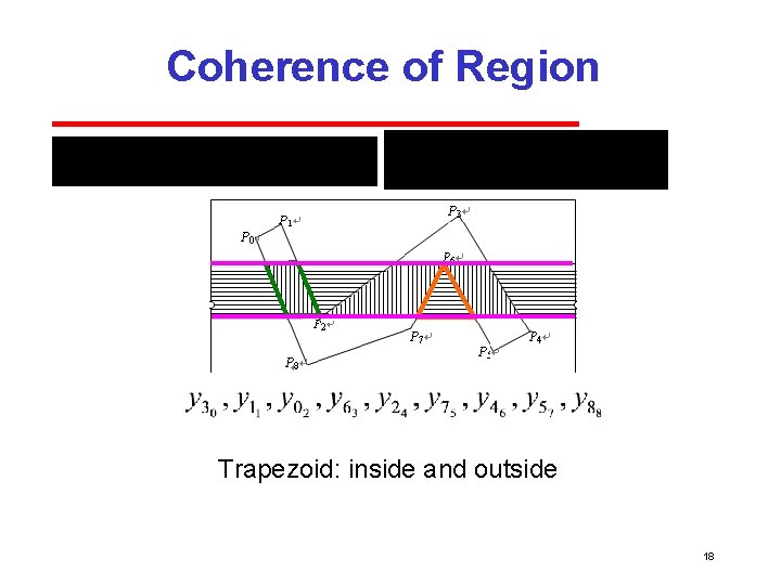
Coherence of Region Trapezoid: inside and outside 18

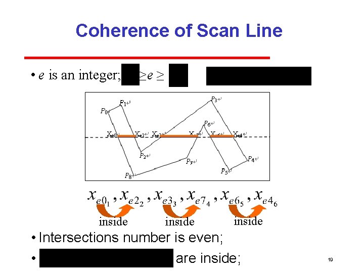
Coherence of Scan Line • e is an integer; inside ≥e ≥ inside • Intersections number is even; • are inside; 19

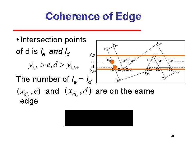
Coherence of Edge • Intersection points of d is le and ld y 63 e d y 24 The number of le = ld and are on the same edge 20

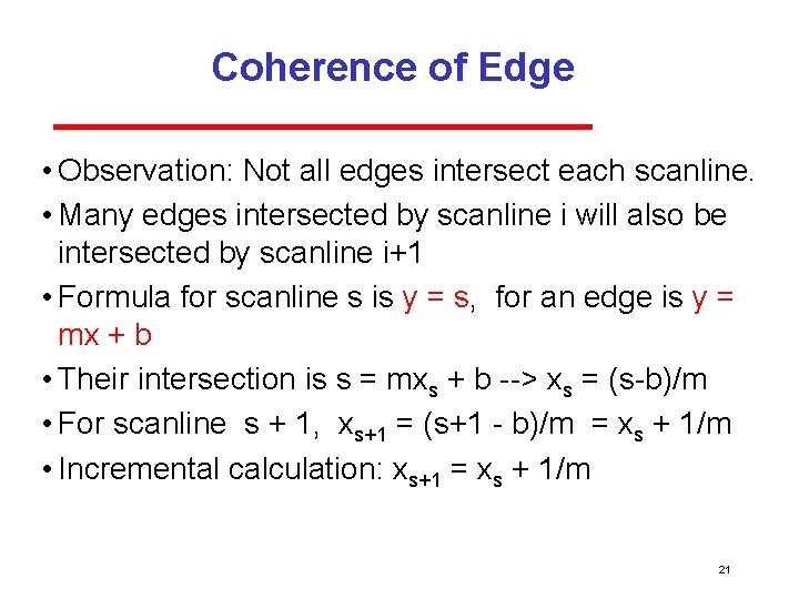
Coherence of Edge • Observation: Not all edges intersect each scanline. • Many edges intersected by scanline i will also be intersected by scanline i+1 • Formula for scanline s is y = s, for an edge is y = mx + b • Their intersection is s = mxs + b > xs = (s b)/m • For scanline s + 1, xs+1 = (s+1 b)/m = xs + 1/m • Incremental calculation: xs+1 = xs + 1/m 21

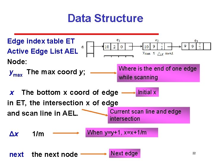
Data Structure Edge index table ET Active Edge List AEL Node: ymax The max coord y; Where is the end of one edge while scanning Initial x x The bottom x coord of edge in ET, the intersection x of edge Current scan line and edge and scan line in AEL. intersection Δx 1/m next the next node When y=y+1, x=x+1/m Next edge 22

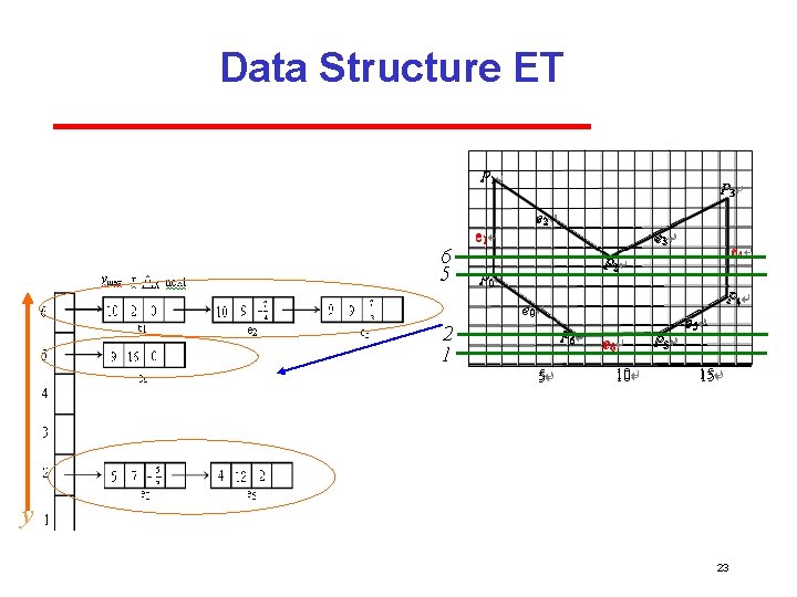
Data Structure ET 6 5 2 1 y 23

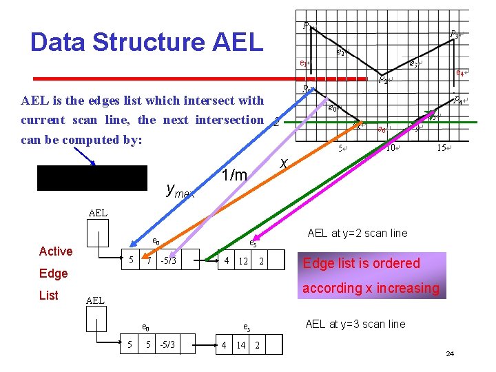
Data Structure AEL is the edges list which intersect with current scan line, the next intersection 2 can be computed by: ymax x 1/m AEL e 0 Active 5 7 -5/3 Edge List AEL at y=2 scan line e 5 4 12 2 Edge list is ordered according x increasing AEL e 0 5 5 -5/3 e 5 4 14 2 AEL at y=3 scan line 24

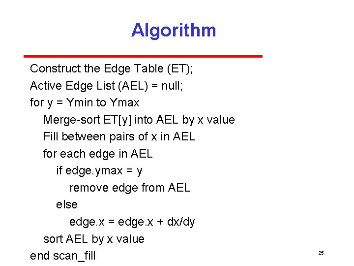
Algorithm Construct the Edge Table (ET); Active Edge List (AEL) = null; for y = Ymin to Ymax Merge sort ET[y] into AEL by x value Fill between pairs of x in AEL for each edge in AEL if edge. ymax = y remove edge from AEL else edge. x = edge. x + dx/dy sort AEL by x value end scan_fill 25

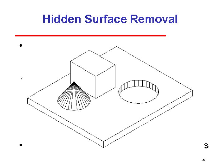
Hidden Surface Removal • Object space approach: use pairwise testing between polygons (objects space) partially obscuring can draw independently • Worst case complexity O(n 2) for n polygons 26

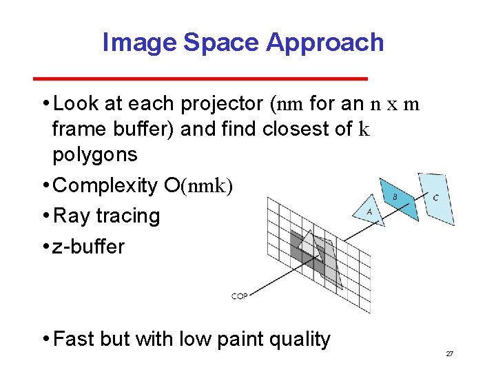
Image Space Approach • Look at each projector (nm for an n x m frame buffer) and find closest of k polygons • Complexity O(nmk) • Ray tracing • z buffer • Fast but with low paint quality 27

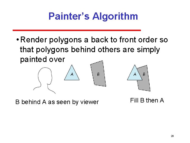
Painter’s Algorithm • Render polygons a back to front order so that polygons behind others are simply painted over B behind A as seen by viewer Fill B then A 28

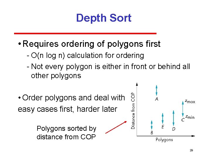
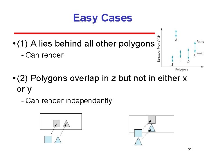
Depth Sort • Requires ordering of polygons first O(n log n) calculation for ordering Not every polygon is either in front or behind all other polygons • Order polygons and deal with easy cases first, harder later Polygons sorted by distance from COP 29

Easy Cases • (1) A lies behind all other polygons Can render • (2) Polygons overlap in z but not in either x or y Can render independently 30

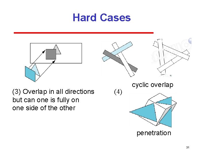
Hard Cases (3) Overlap in all directions but can one is fully on one side of the other (4) cyclic overlap penetration 31

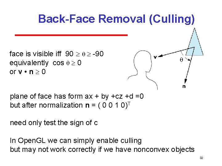
Back-Face Removal (Culling) face is visible iff 90 equivalently cos 0 or v • n 0 plane of face has form ax + by +cz +d =0 but after normalization n = ( 0 0 1 0)T need only test the sign of c In Open. GL we can simply enable culling but may not work correctly if we have nonconvex objects 32

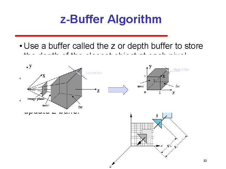
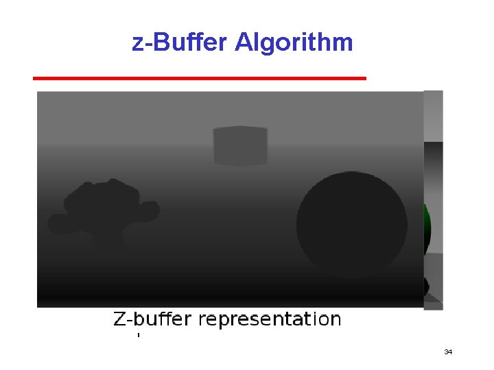
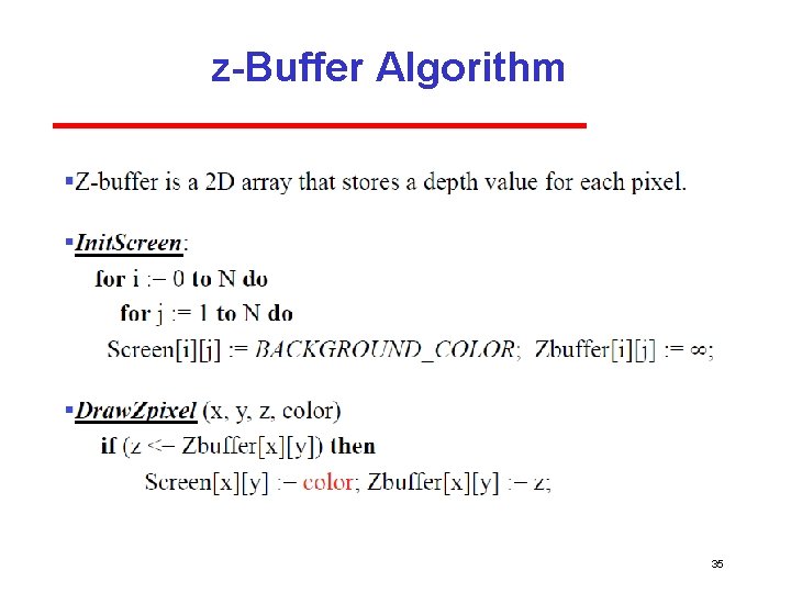
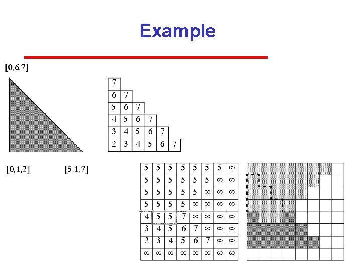
z-Buffer Algorithm • Use a buffer called the z or depth buffer to store the depth of the closest object at each pixel found so far • As we render each polygon, compare the depth of each pixel to depth in z buffer • If less, place shade of pixel in color buffer and update z buffer 33

z-Buffer Algorithm 34

z-Buffer Algorithm 35

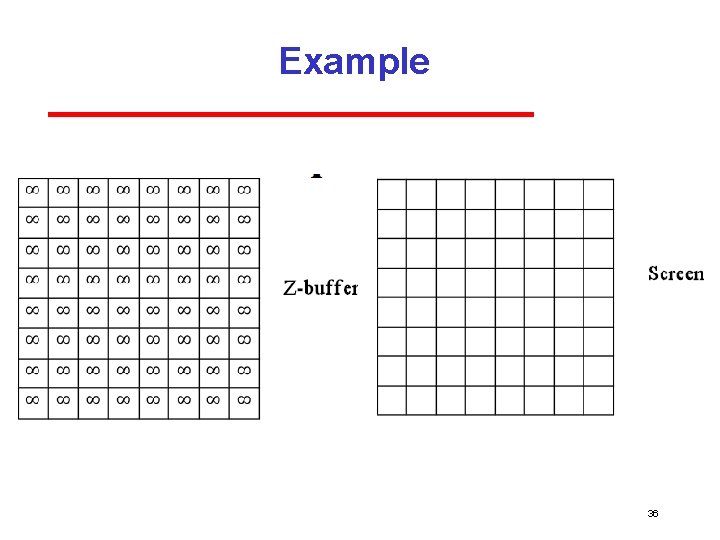
Example 36

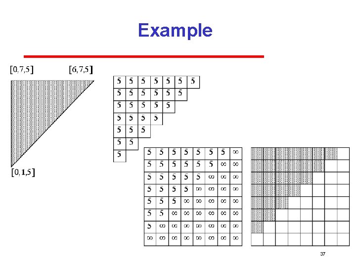
Example 37

Example 38

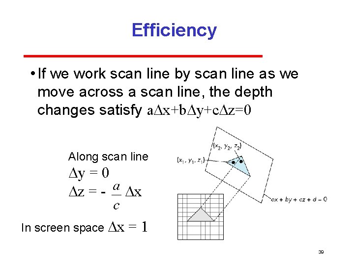
Efficiency • If we work scan line by scan line as we move across a scan line, the depth changes satisfy a x+b y+c z=0 Along scan line y = 0 z = - In screen space x x =1 39

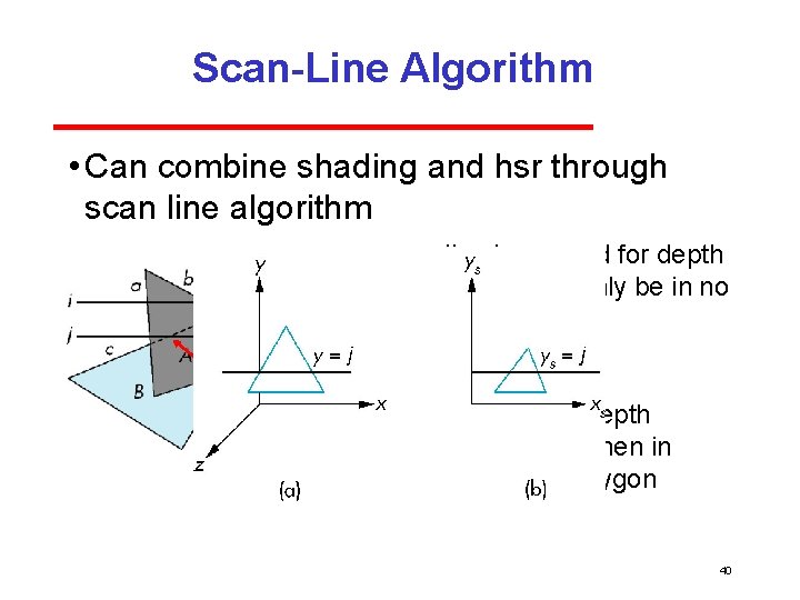
Scan-Line Algorithm • Can combine shading and hsr through scan line algorithm scan line i: no need for depth information, can only be in no or one polygon scan line j: need depth information only when in more than one polygon 40

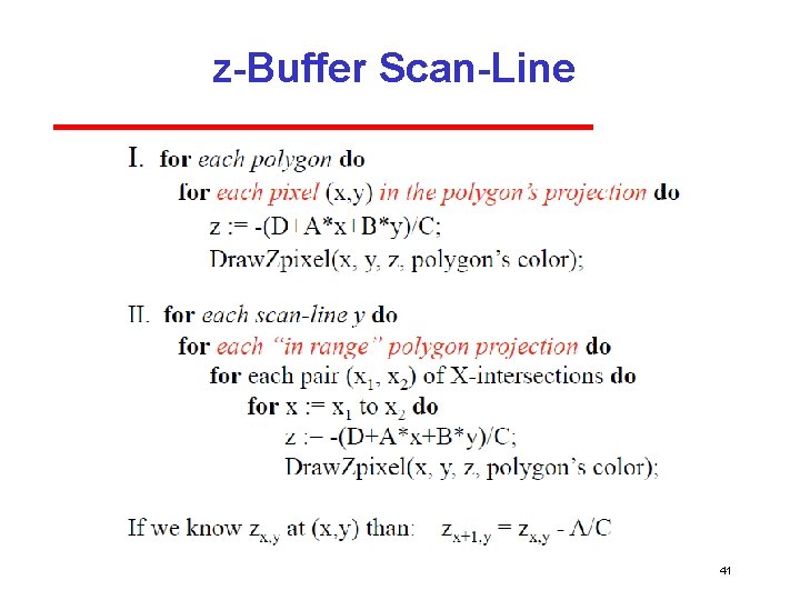
z-Buffer Scan-Line 41

Implementation • Need a data structure to store Flag for each polygon (inside/outside) Incremental structure for scan lines that stores which edges are encountered Parameters for planes for intersections 42

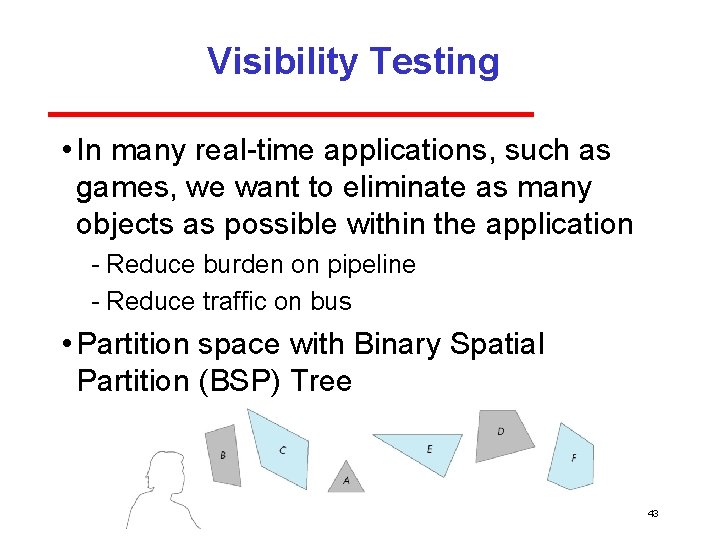
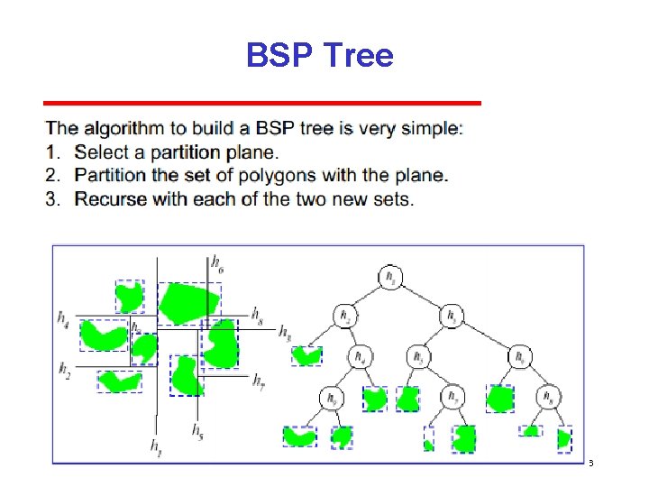
Visibility Testing • In many real time applications, such as games, we want to eliminate as many objects as possible within the application Reduce burden on pipeline Reduce traffic on bus • Partition space with Binary Spatial Partition (BSP) Tree 43

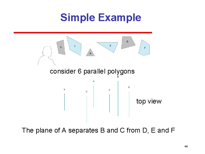
Simple Example consider 6 parallel polygons top view The plane of A separates B and C from D, E and F 44

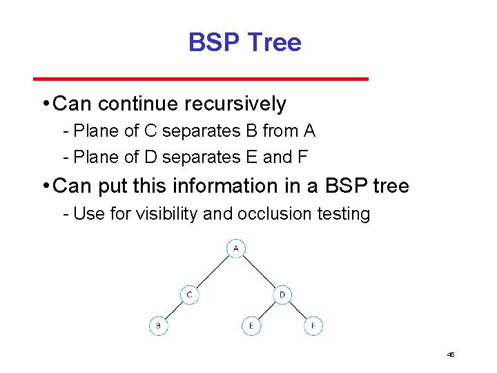
BSP Tree • Can continue recursively Plane of C separates B from A Plane of D separates E and F • Can put this information in a BSP tree Use for visibility and occlusion testing 45

BSP Tree 46

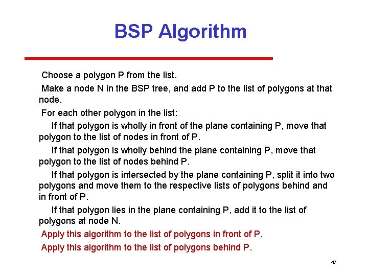
BSP Algorithm Choose a polygon P from the list. Make a node N in the BSP tree, and add P to the list of polygons at that node. For each other polygon in the list: If that polygon is wholly in front of the plane containing P, move that polygon to the list of nodes in front of P. If that polygon is wholly behind the plane containing P, move that polygon to the list of nodes behind P. If that polygon is intersected by the plane containing P, split it into two polygons and move them to the respective lists of polygons behind and in front of P. If that polygon lies in the plane containing P, add it to the list of polygons at node N. Apply this algorithm to the list of polygons in front of P. Apply this algorithm to the list of polygons behind P. 47

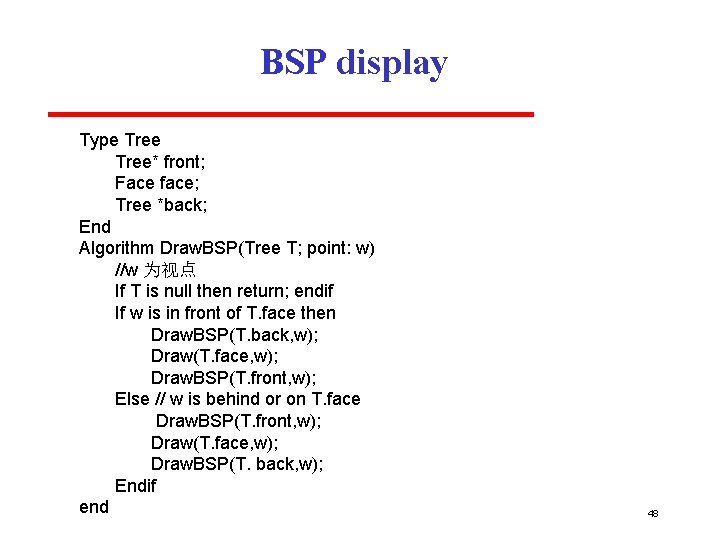
BSP display Type Tree* front; Face face; Tree *back; End Algorithm Draw. BSP(Tree T; point: w) //w 为视点 If T is null then return; endif If w is in front of T. face then Draw. BSP(T. back, w); Draw(T. face, w); Draw. BSP(T. front, w); Else // w is behind or on T. face Draw. BSP(T. front, w); Draw(T. face, w); Draw. BSP(T. back, w); Endif end 48

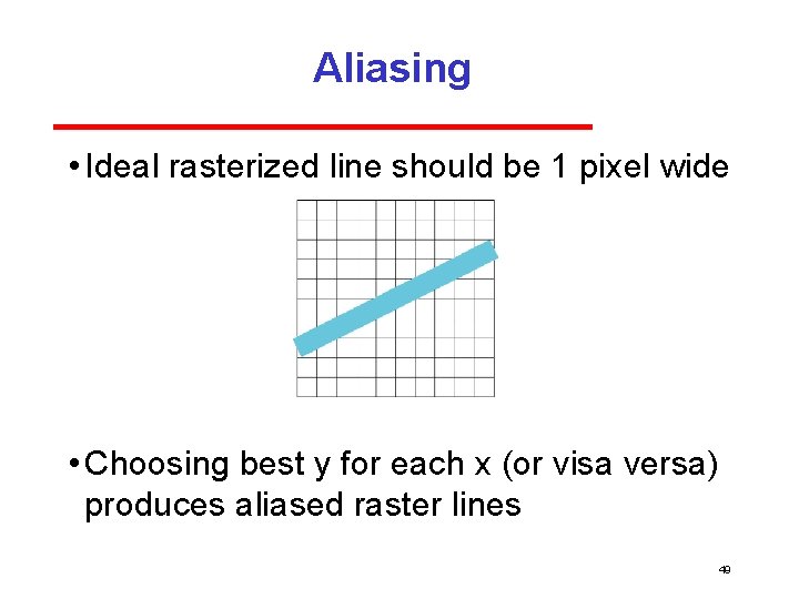
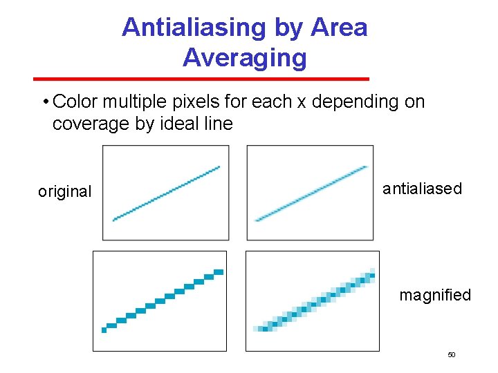
Aliasing • Ideal rasterized line should be 1 pixel wide • Choosing best y for each x (or visa versa) produces aliased raster lines 49

Antialiasing by Area Averaging • Color multiple pixels for each x depending on coverage by ideal line original antialiased magnified 50

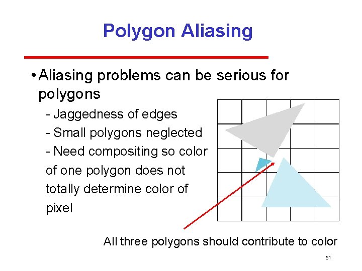
Polygon Aliasing • Aliasing problems can be serious for polygons Jaggedness of edges Small polygons neglected Need compositing so color of one polygon does not totally determine color of pixel All three polygons should contribute to color 51

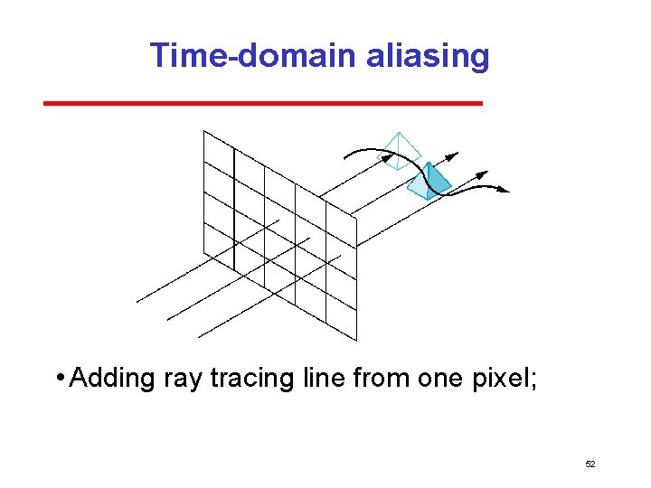
Time-domain aliasing • Adding ray tracing line from one pixel; 52