First Order Linear Differential Equations Any equation containing

First Order Linear Differential Equations Any equation containing a derivative is called a differential equation. A function which satisfies the equation is called a solution to the differential equation. The order of the differential equation is the order of the highest derivative involved. The degree of the differential equation is the degree of the power of the highest derivative involved. We can then integrate both sides. This will obtain the general solution.

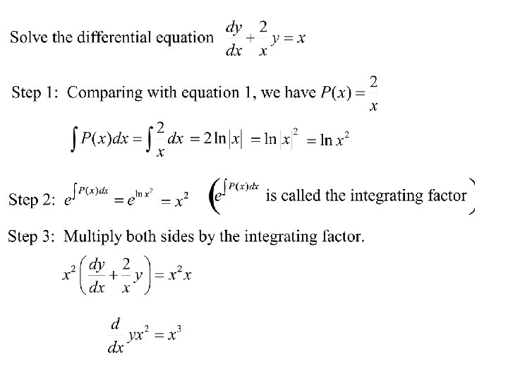
A first order linear differential equation is an equation of the form 1 To find a method for solving this equation, lets consider the simpler equation Which can be solved by separating the variables. (Remember: a solution is of the form y = f(x) )

or Using the product rule to differentiate the LHS we get:

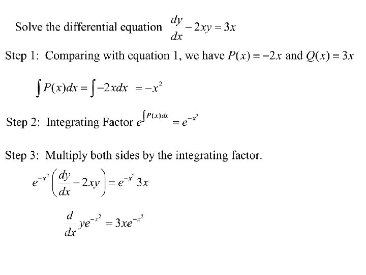
Returning to equation 1, If we multiply both sides by Now integrate both sides. For this to work we need to be able to find

Note the solution is composed of two parts. The particular solution satisfies the equation: The complementary function satisfies the equation:

To solve this integration we need to use substitution. If you look at page 113 you will see a note regarding the constant when finding the integrating factor. We need not find it as it cancels out when we multiply both sides of the equation.

The modulus vanishes as we will have either both positive on either side or both negative. Their effect is cancelled. (note the shortcut I have taken here)

(note the shortcut I have taken here) The modulus vanishes as we will have either both positive on either side or both negative. Their effect is cancelled.

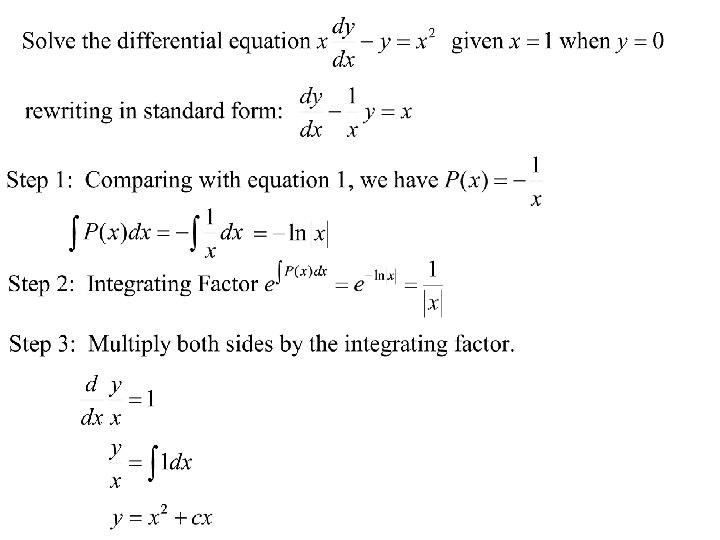
So far we have looked at the general solutions only. They represent a whole family of curves. If one point can be found which lies on the desired curve, then a unique solution can be identified. Such a point is often given and its coordinates are referred to as the initial conditions or values. The unique solution is called a particular solution.

Hence the particular solution is Page 114 and 116 Exercise 1 and 2 TJ Exercise 1

Second-order linear differential equations Note that the general solution to such an equation must include two arbitrary constants to be completely general.

Proof Adding:

The solutions to this quadratic will provide two values of m which will make y = Aemx a solution.

If we call these two values m 1 and m 2, then we have two solutions. and A and B are used to distinguish the two arbitrary constants. Is a solution. The two arbitrary constants needed for second order differential equations ensure all solutions are covered. The type of solution we get depends on the nature of the roots of this equation.

When roots are real and distinct The auxiliary equation is To find a particular solution we must be given enough information.

The auxiliary equation is Using the initial conditions.

Solving gives Thus the particular solution is Page 119 Exercise 3 Questions 1(a), (b) 2(a), (b) But we will now look at the solution when the roots are real and coincident.

Roots are real and coincident When the roots of the auxiliary equation are both real and equal to m, then the solution would appear to be y = Aemx + Bemx = (A+B)emx A + B however is equivalent to a single constant and second order equations need two. With a little further searching we find that y = Bxemx is a solution. Proof on p 119 So a general solution is

The auxiliary equation is

The auxiliary equation is Using the initial conditions.

Page 120 Exercise 4 Questions 1(a), (b) 2(a), (b) But we will now look at the solution when the roots are complex conjugates.

Roots are complex conjugates When the roots of the auxiliary equation are complex, they will be of the form m 1 = p + iq and m 2 = p – iq. Hence the general equation will be

The auxiliary equation is

The auxiliary equation is Substituting gives:

Substituting gives: The particular solution is Page 122 Exercise 5 A Questions 1(a), (b) 2(a), (b) TJ Exercise 2

Non homogeneous second order differential equations Non homogeneous equations take the form Suppose g(x) is a particular solution to this equation. Then Now suppose that g(x) + k(x) is another solution. Then

Giving From the work in previous exercises we know how to find k(x). This function is referred to as the Complimentary Function. (CF) The function g(x) is referred to as the Particular Integral. (PI) General Solution = CF + PI

Finding the (CF): the auxiliary equation is Substituting into the original equation

Hence the general solution is

Finding the (CF): the auxiliary equation is Substituting into the original equation

Hence the general solution is

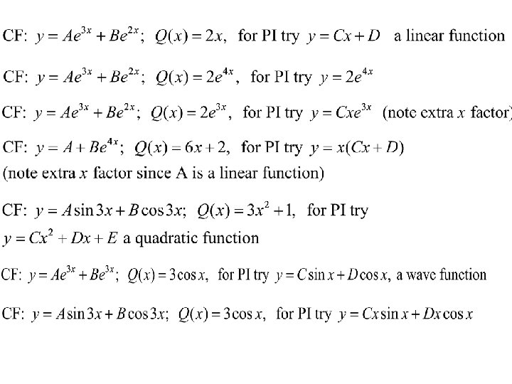
Finding the form of the PI The individual terms of the CF make the LHS zero The PI makes the LHS equal to Q(x). Since Q(x) ≠ 0, it stands to reason that the PI cannot have the same form as the CF. When choosing the form of the PI, we usually select the same form as Q(x). This reasoning leads us to select the PI according to the following steps. • try the same form as Q(x) • If this is the same form as a term of the CF, then try x 2 Q(x)

Finding the (CF): the auxiliary equation is Substituting into the original equation

If the wrong selection of PI is made, you will generally be alerted to this by the occurrence of some contradiction in later work. Page 126 – Exercise 7 A as many as possible. TJ Exercise 3. This assesses beyond poly and trig work.