Differential Equations 7 7 5 The Logistic Equation

Differential Equations 7

7. 5 The Logistic Equation

The Logistic Model 3

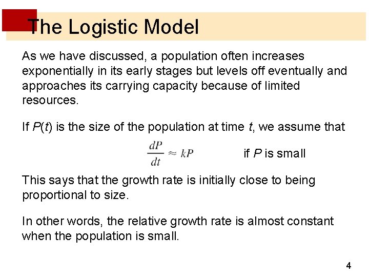
The Logistic Model As we have discussed, a population often increases exponentially in its early stages but levels off eventually and approaches its carrying capacity because of limited resources. If P(t) is the size of the population at time t, we assume that if P is small This says that the growth rate is initially close to being proportional to size. In other words, the relative growth rate is almost constant when the population is small. 4

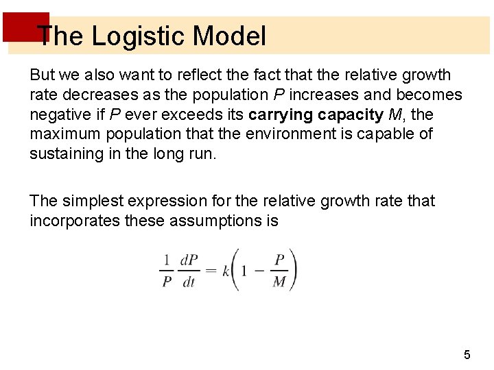
The Logistic Model But we also want to reflect the fact that the relative growth rate decreases as the population P increases and becomes negative if P ever exceeds its carrying capacity M, the maximum population that the environment is capable of sustaining in the long run. The simplest expression for the relative growth rate that incorporates these assumptions is 5

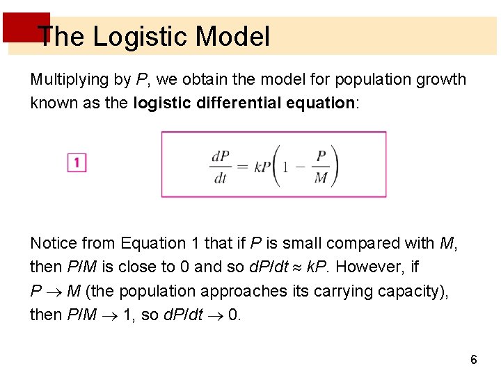
The Logistic Model Multiplying by P, we obtain the model for population growth known as the logistic differential equation: Notice from Equation 1 that if P is small compared with M, then P/M is close to 0 and so d. P/dt k. P. However, if P M (the population approaches its carrying capacity), then P/M 1, so d. P/dt 0. 6

The Logistic Model We can deduce information about whether solutions increase or decrease directly from Equation 1. If the population P lies between 0 and M, then the right side of the equation is positive, so d. P/dt > 0 and the population increases. But if the population exceeds the carrying capacity (P > M), then 1 – P/M is negative, so d. P/dt < 0 and the population decreases. 7

Direction Fields 8

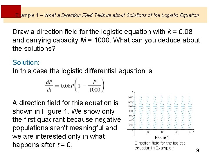
Example 1 – What a Direction Field Tells us about Solutions of the Logistic Equation Draw a direction field for the logistic equation with k = 0. 08 and carrying capacity M = 1000. What can you deduce about the solutions? Solution: In this case the logistic differential equation is A direction field for this equation is shown in Figure 1. We show only the first quadrant because negative populations aren’t meaningful and we are interested only in what happens after t = 0. Figure 1 Direction field for the logistic equation in Example 1 9

Example 1 – Solution cont’d The logistic equation is autonomous (d. P/dt depends only on P, not on t), so the slopes are the same along any horizontal line. As expected, the slopes are positive for 0 < P < 1000 and negative for P > 1000. The slopes are small when P is close to 0 or 1000 (the carrying capacity). Notice that the solutions move away from the equilibrium solution P = 0 and move toward the equilibrium solution P = 1000. 10

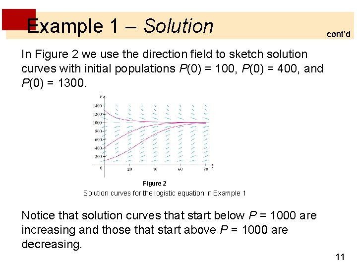
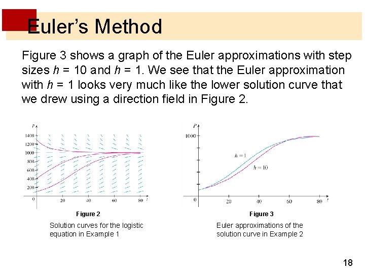
Example 1 – Solution cont’d In Figure 2 we use the direction field to sketch solution curves with initial populations P(0) = 100, P(0) = 400, and P(0) = 1300. Figure 2 Solution curves for the logistic equation in Example 1 Notice that solution curves that start below P = 1000 are increasing and those that start above P = 1000 are decreasing. 11

Example 1 – Solution cont’d The slopes are greatest when P 500 and therefore the solution curves that start below P = 1000 have inflection points when P 500. In fact we can prove that all solution curves that start below P = 500 have an inflection point when P is exactly 500. 12

Euler’s Method 13

Euler’s Method Let’s use Euler’s method to obtain numerical estimates for solutions of the logistic differential equation at specific times. 14

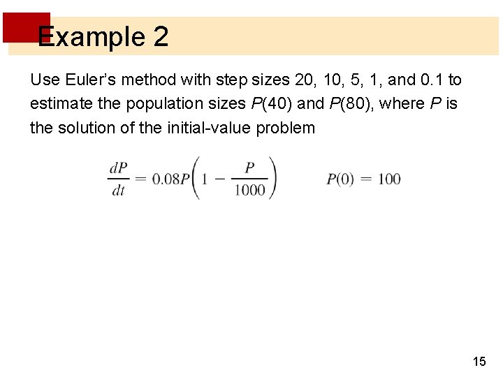
Example 2 Use Euler’s method with step sizes 20, 10, 5, 1, and 0. 1 to estimate the population sizes P(40) and P(80), where P is the solution of the initial-value problem 15

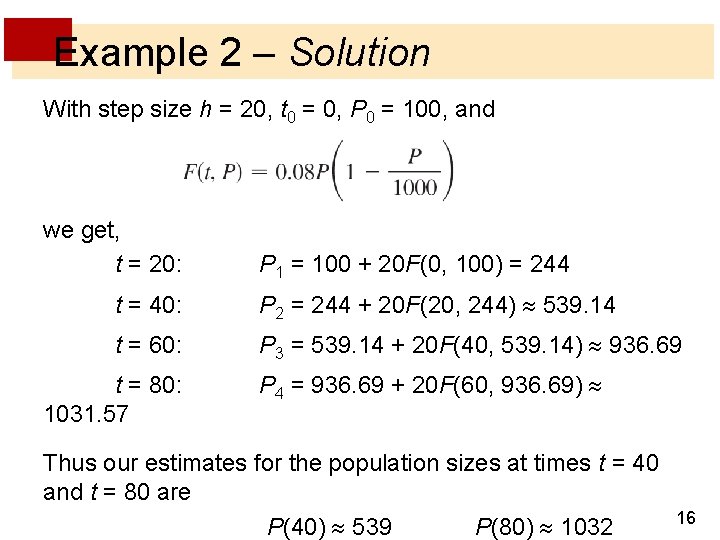
Example 2 – Solution With step size h = 20, t 0 = 0, P 0 = 100, and we get, t = 20: P 1 = 100 + 20 F(0, 100) = 244 t = 40: P 2 = 244 + 20 F(20, 244) 539. 14 t = 60: P 3 = 539. 14 + 20 F(40, 539. 14) 936. 69 t = 80: 1031. 57 P 4 = 936. 69 + 20 F(60, 936. 69) Thus our estimates for the population sizes at times t = 40 and t = 80 are P(40) 539 P(80) 1032 16

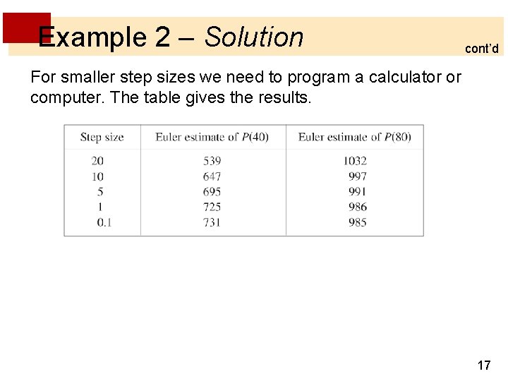
Example 2 – Solution cont’d For smaller step sizes we need to program a calculator or computer. The table gives the results. 17

Euler’s Method Figure 3 shows a graph of the Euler approximations with step sizes h = 10 and h = 1. We see that the Euler approximation with h = 1 looks very much like the lower solution curve that we drew using a direction field in Figure 2 Solution curves for the logistic equation in Example 1 Figure 3 Euler approximations of the solution curve in Example 2 18

The Analytic Solution 19

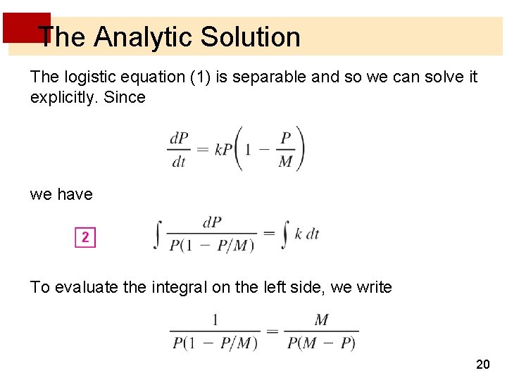
The Analytic Solution The logistic equation (1) is separable and so we can solve it explicitly. Since we have To evaluate the integral on the left side, we write 20

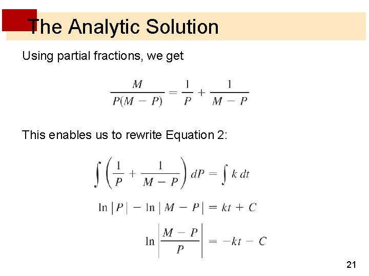
The Analytic Solution Using partial fractions, we get This enables us to rewrite Equation 2: 21

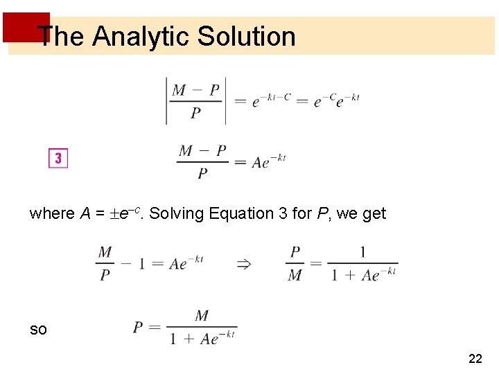
The Analytic Solution where A = e–c. Solving Equation 3 for P, we get so 22

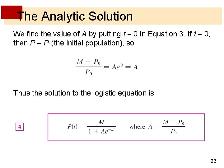
The Analytic Solution We find the value of A by putting t = 0 in Equation 3. If t = 0, then P = P 0(the initial population), so Thus the solution to the logistic equation is 23

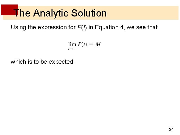
The Analytic Solution Using the expression for P(t) in Equation 4, we see that which is to be expected. 24

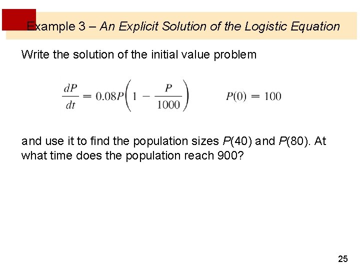
Example 3 – An Explicit Solution of the Logistic Equation Write the solution of the initial value problem and use it to find the population sizes P(40) and P(80). At what time does the population reach 900? 25

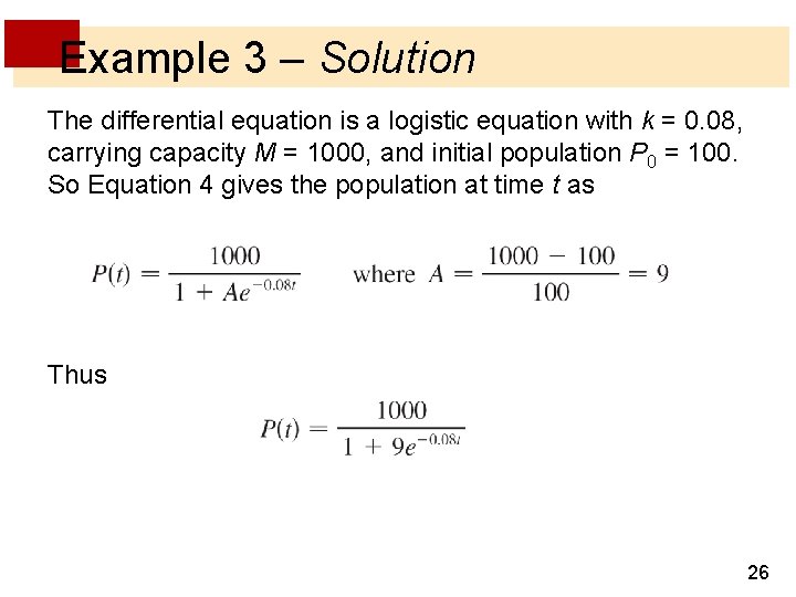
Example 3 – Solution The differential equation is a logistic equation with k = 0. 08, carrying capacity M = 1000, and initial population P 0 = 100. So Equation 4 gives the population at time t as Thus 26

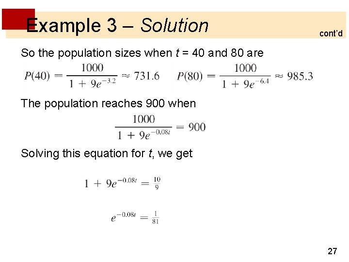
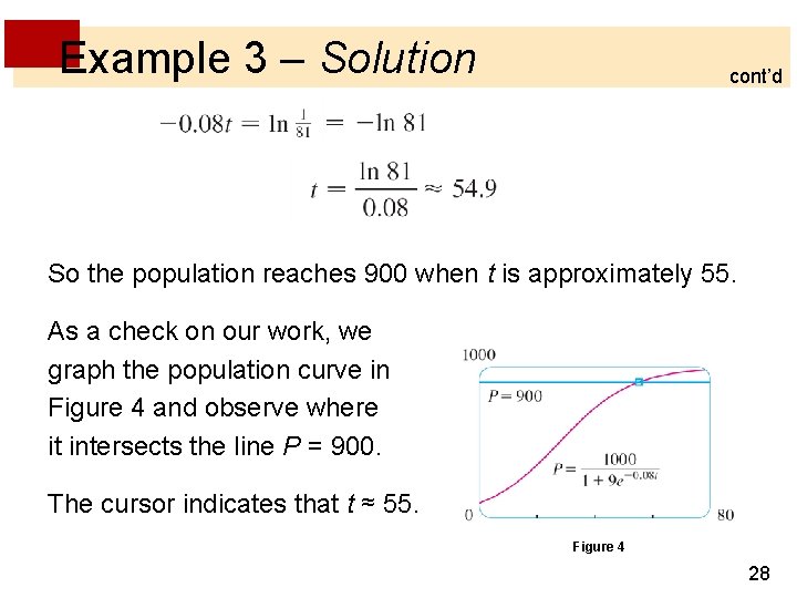
Example 3 – Solution cont’d So the population sizes when t = 40 and 80 are The population reaches 900 when Solving this equation for t, we get 27

Example 3 – Solution cont’d So the population reaches 900 when t is approximately 55. As a check on our work, we graph the population curve in Figure 4 and observe where it intersects the line P = 900. The cursor indicates that t ≈ 55. Figure 4 28

Comparison of the Natural Growth and Logistic Models 29

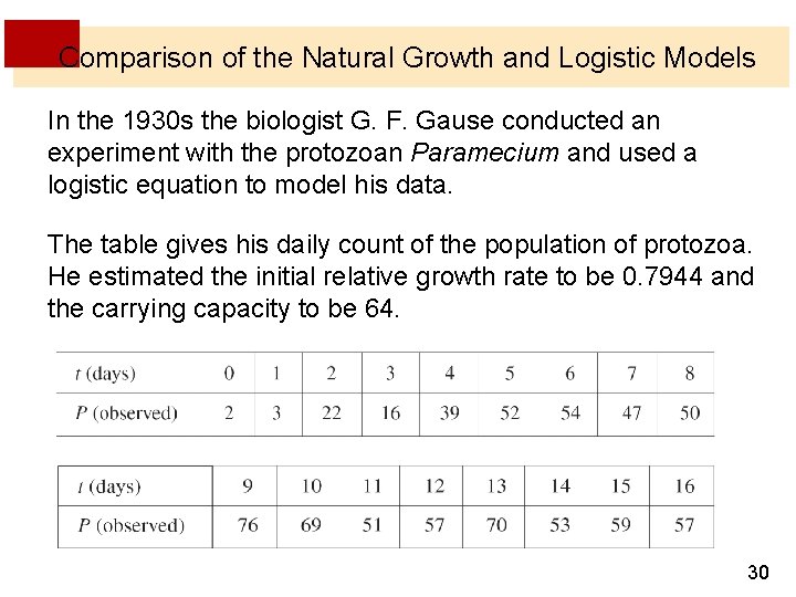
Comparison of the Natural Growth and Logistic Models In the 1930 s the biologist G. F. Gause conducted an experiment with the protozoan Paramecium and used a logistic equation to model his data. The table gives his daily count of the population of protozoa. He estimated the initial relative growth rate to be 0. 7944 and the carrying capacity to be 64. 30

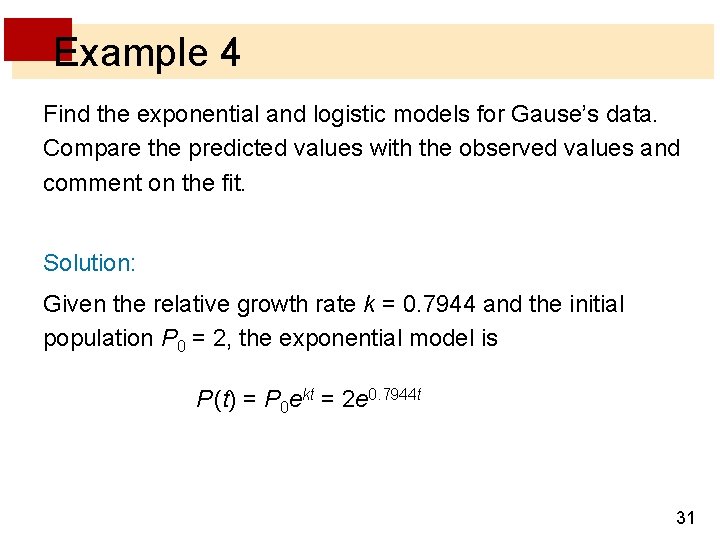
Example 4 Find the exponential and logistic models for Gause’s data. Compare the predicted values with the observed values and comment on the fit. Solution: Given the relative growth rate k = 0. 7944 and the initial population P 0 = 2, the exponential model is P (t) = P 0 ekt = 2 e 0. 7944 t 31

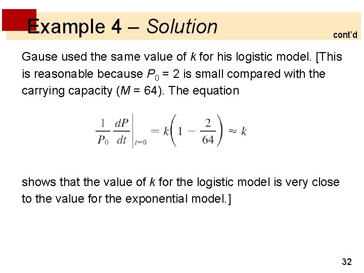
Example 4 – Solution cont’d Gause used the same value of k for his logistic model. [This is reasonable because P 0 = 2 is small compared with the carrying capacity (M = 64). The equation shows that the value of k for the logistic model is very close to the value for the exponential model. ] 32

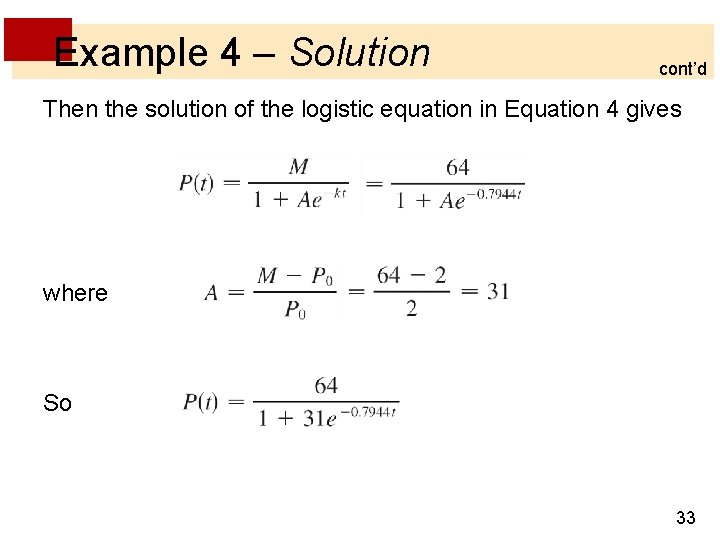
Example 4 – Solution cont’d Then the solution of the logistic equation in Equation 4 gives where So 33

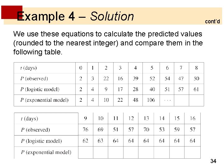
Example 4 – Solution cont’d We use these equations to calculate the predicted values (rounded to the nearest integer) and compare them in the following table. 34

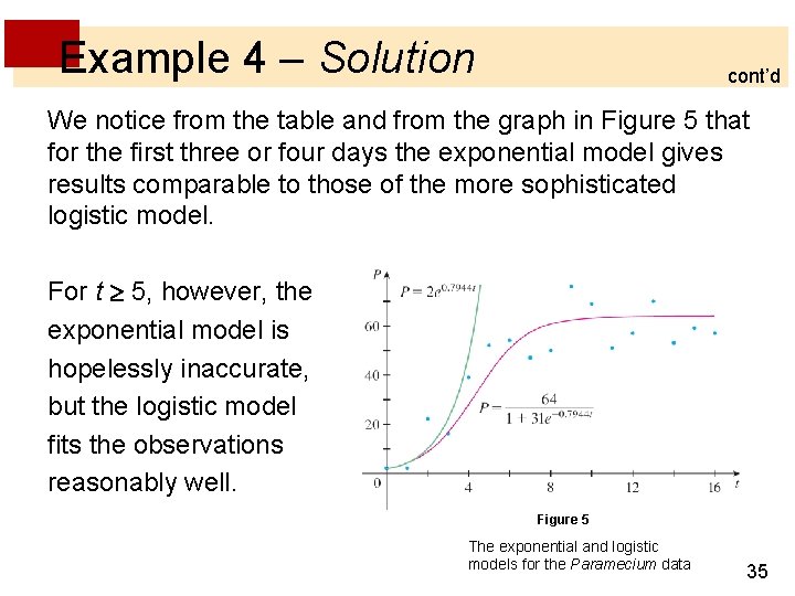
Example 4 – Solution cont’d We notice from the table and from the graph in Figure 5 that for the first three or four days the exponential model gives results comparable to those of the more sophisticated logistic model. For t 5, however, the exponential model is hopelessly inaccurate, but the logistic model fits the observations reasonably well. Figure 5 The exponential and logistic models for the Paramecium data 35

Other Models for Population Growth 36

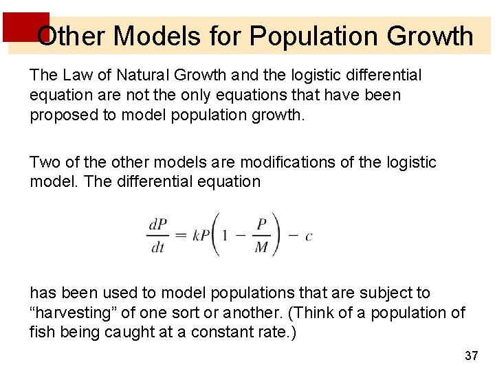
Other Models for Population Growth The Law of Natural Growth and the logistic differential equation are not the only equations that have been proposed to model population growth. Two of the other models are modifications of the logistic model. The differential equation has been used to model populations that are subject to “harvesting” of one sort or another. (Think of a population of fish being caught at a constant rate. ) 37

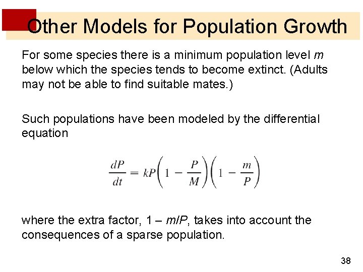
Other Models for Population Growth For some species there is a minimum population level m below which the species tends to become extinct. (Adults may not be able to find suitable mates. ) Such populations have been modeled by the differential equation where the extra factor, 1 – m/P, takes into account the consequences of a sparse population. 38