Lecture 28 Linear Differential Equations Last Lecture Summary


 Linear")


 Integrating (1), we obtain")
 K > 0, for growth K < 0, for decay C is an")
 Solution: We first solve the differential equation …………………. . (1)")


 takes the form at , we")


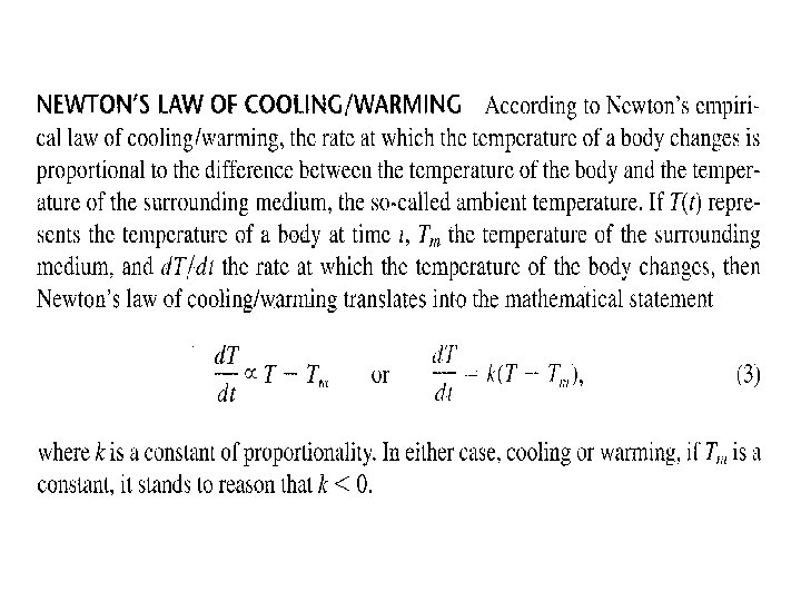
 When a cake is removed from an oven, its")


- Slides: 40
Lecture 28 Linear Differential Equations
Last Lecture Summary Last time, we covered the topic: Separable Differential Equations • Separable Equations • Method of Solution
Today We will cover the topic: • Linear Differential Equations • Applications of Differential Equation – Mathematical Modeling
Linear Equations An equation of the form is called a (1 st Order) Linear Differential Equation. 1 st Order – because the highest derivative appearing in the equation is of order 1.
The equation can be rewritten in the following famous form where and are continuous functions.
6
Method of solution The general solution of the first order linear differential equation is given by The function is called the integrating factor. If there is an IC given, then we use it to find the constant C. 7
Summary: 1. Identify that the equation is 1 st order linear equation. Rewrite it in the form if the equation is not already in this form. 2. Find the integrating factor
3. Write down the general solution 4. If you are given an IVP, use the initial condition to find the constant C. 5. Plug in the calculated value to write the particular solution of the problem.
Example Solve Solution: This is already in the standard form Where and
Now the integrating factor is Multiplying with the , we get
Example Solve 14
Modeling with Differential Equations By the term mathematical modeling we mean the process whereby the behavior of a real – life system or phenomenon, whether physical, sociological, or even economics is described by a set of mathematical relations, after approximation and idealizations. Construction of mathematical model starts with
1. Identification of the system for modeling. This requires selection of some variables as important to understanding or describing the behavior of the system and ignoring other as marginal or irrelevant to this understanding. 2. Making some realistic assumption, or hypothesis, about the system we are describing. These assumptions will also include any empirical laws that may be applicable of the system.
3. Modeling steps are the steps that lead from the physical situation to a mathematical formulation and solution, then physical interpretation of the result. Now, let’s solve some models that are described by linear first order differential equations.
Growth and Decay : •
Step 2: Solving the differential equation obtained ………………. . (1) Integrating (1), we obtain
…………………(2) K > 0, for growth K < 0, for decay C is an arbitrary constant and can be determined by using initial condition and value of k changes from problem to problem. Step 3: Interpretation of the result.
Example (Bacterial Growth) Solution: We first solve the differential equation …………………. . (1)
Subject to . Then we use the empirical condition to determine the constant of proportionality k. Now Eq. (1) is both separable and linear. When it is put into the form ……. . . (2) We can see by inspection that the integrating factor is . Multiplying (2) with , we get ………………. (3) Integrating (3) ………………. (4)
It follows from , that so equation (4) takes the form at , we have ………………. (5)
Thus To find the time at which the bacteria have tripled we solve
Example (Cooling of a Cake) When a cake is removed from an oven, its temperature is measured at 300 o. F. Three minutes later its temperature is 200 o. F. How long will it take for the cake to cool off to a room temperature of 70 o. F? Solution:
Review We covered the topic: • Linear Differential Equations • Applications of Differential Equations – Mathematical Modelig Next time, we will start Chapter 20: Functions of Several Variables 40