ELEC 5200 0016200 001 Computer Architecture and Design

ELEC 5200 -001/6200 -001 Computer Architecture and Design Spring 2015 Performance of a Computer (Chapter 4) Vishwani D. Agrawal James J. Danaher Professor Department of Electrical and Computer Engineering Auburn University, Auburn, AL 36849 http: //www. eng. auburn. edu/~vagrawal@eng. auburn. edu Spr 2015, Apr 13. . . ELEC 5200 -001/6200 -001 Lecture 10 1

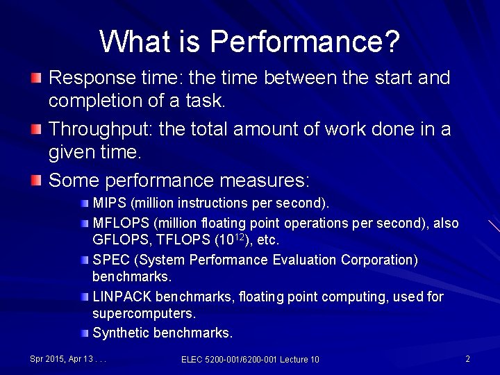
What is Performance? Response time: the time between the start and completion of a task. Throughput: the total amount of work done in a given time. Some performance measures: MIPS (million instructions per second). MFLOPS (million floating point operations per second), also GFLOPS, TFLOPS (1012), etc. SPEC (System Performance Evaluation Corporation) benchmarks. LINPACK benchmarks, floating point computing, used for supercomputers. Synthetic benchmarks. Spr 2015, Apr 13. . . ELEC 5200 -001/6200 -001 Lecture 10 2

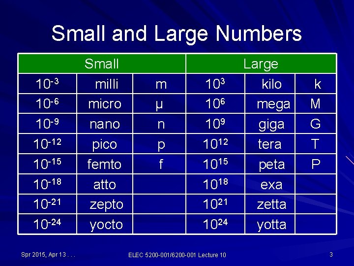
Small and Large Numbers 10 -3 10 -6 10 -9 10 -12 10 -15 10 -18 10 -21 10 -24 Spr 2015, Apr 13. . . Small milli micro nano pico femto atto zepto yocto m μ n p f 103 106 109 1012 1015 1018 1021 1024 ELEC 5200 -001/6200 -001 Lecture 10 Large kilo mega giga tera peta exa zetta yotta k M G T P 3

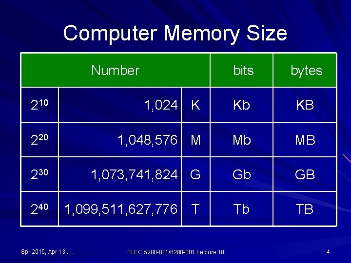
Computer Memory Size Number bits bytes 210 1, 024 K Kb KB 220 1, 048, 576 M Mb MB 230 1, 073, 741, 824 G Gb GB 240 1, 099, 511, 627, 776 T Tb TB Spr 2015, Apr 13. . . ELEC 5200 -001/6200 -001 Lecture 10 4

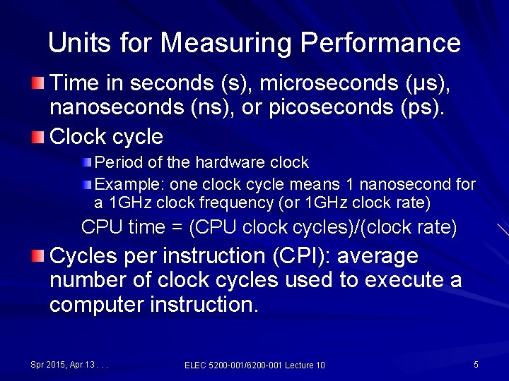
Units for Measuring Performance Time in seconds (s), microseconds (μs), nanoseconds (ns), or picoseconds (ps). Clock cycle Period of the hardware clock Example: one clock cycle means 1 nanosecond for a 1 GHz clock frequency (or 1 GHz clock rate) CPU time = (CPU clock cycles)/(clock rate) Cycles per instruction (CPI): average number of clock cycles used to execute a computer instruction. Spr 2015, Apr 13. . . ELEC 5200 -001/6200 -001 Lecture 10 5

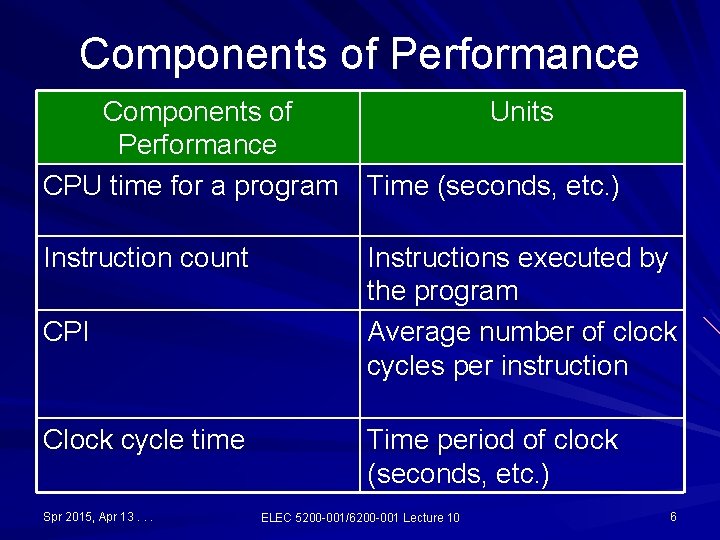
Components of Performance Components of Units Performance CPU time for a program Time (seconds, etc. ) Instruction count CPI Clock cycle time Spr 2015, Apr 13. . . Instructions executed by the program Average number of clock cycles per instruction Time period of clock (seconds, etc. ) ELEC 5200 -001/6200 -001 Lecture 10 6

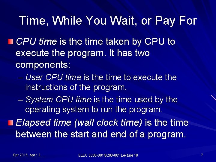
Time, While You Wait, or Pay For CPU time is the time taken by CPU to execute the program. It has two components: – User CPU time is the time to execute the instructions of the program. – System CPU time is the time used by the operating system to run the program. Elapsed time (wall clock time) is the time between the start and end of a program. Spr 2015, Apr 13. . . ELEC 5200 -001/6200 -001 Lecture 10 7

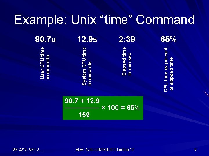
12. 9 s 2: 39 65% Elapsed time In min: sec CPU time as percent of elapsed time User CPU time in seconds 90. 7 u System CPU time in seconds Example: Unix “time” Command 90. 7 + 12. 9 ─────── × 100 = 65% 159 Spr 2015, Apr 13. . . ELEC 5200 -001/6200 -001 Lecture 10 8

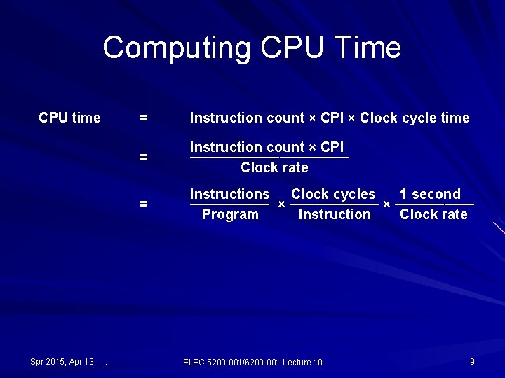
Computing CPU Time CPU time Spr 2015, Apr 13. . . = Instruction count × CPI × Clock cycle time = Instruction count × CPI ──────── Clock rate = Instructions Clock cycles 1 second ──────── × ──────── Program Instruction Clock rate ELEC 5200 -001/6200 -001 Lecture 10 9

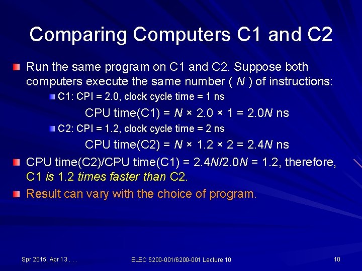
Comparing Computers C 1 and C 2 Run the same program on C 1 and C 2. Suppose both computers execute the same number ( N ) of instructions: C 1: CPI = 2. 0, clock cycle time = 1 ns CPU time(C 1) = N × 2. 0 × 1 = 2. 0 N ns C 2: CPI = 1. 2, clock cycle time = 2 ns CPU time(C 2) = N × 1. 2 × 2 = 2. 4 N ns CPU time(C 2)/CPU time(C 1) = 2. 4 N/2. 0 N = 1. 2, therefore, C 1 is 1. 2 times faster than C 2. Result can vary with the choice of program. Spr 2015, Apr 13. . . ELEC 5200 -001/6200 -001 Lecture 10 10

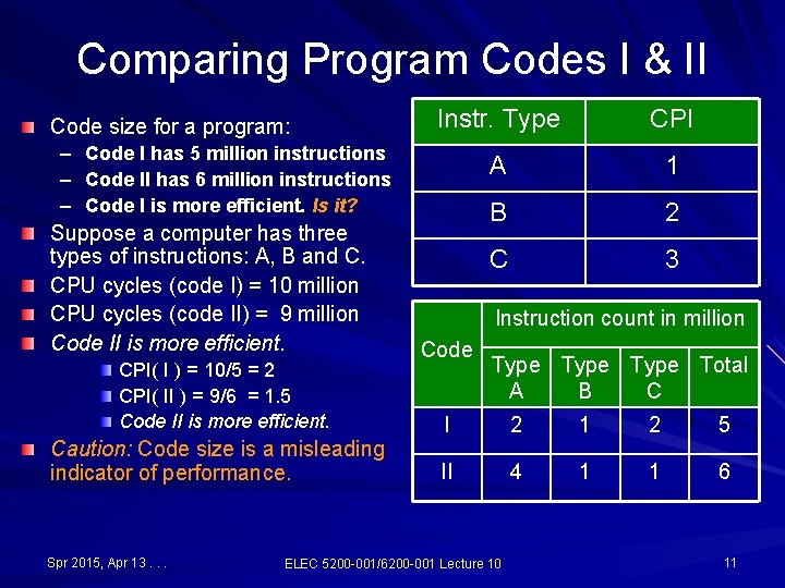
Comparing Program Codes I & II Code size for a program: – – – Instr. Type CPI A 1 B 2 C 3 Code I has 5 million instructions Code II has 6 million instructions Code I is more efficient. Is it? Suppose a computer has three types of instructions: A, B and C. CPU cycles (code I) = 10 million CPU cycles (code II) = 9 million Code II is more efficient. CPI( I ) = 10/5 = 2 CPI( II ) = 9/6 = 1. 5 Code II is more efficient. Caution: Code size is a misleading indicator of performance. Spr 2015, Apr 13. . . Instruction count in million Code Type Total A B C I 2 1 2 5 II 4 1 1 6 ELEC 5200 -001/6200 -001 Lecture 10 11

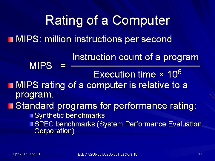
Rating of a Computer MIPS: million instructions per second Instruction count of a program MIPS = ────────── Execution time × 106 MIPS rating of a computer is relative to a program. Standard programs for performance rating: Synthetic benchmarks SPEC benchmarks (System Performance Evaluation Corporation) Spr 2015, Apr 13. . . ELEC 5200 -001/6200 -001 Lecture 10 12

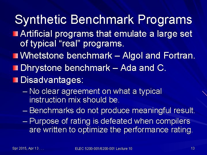
Synthetic Benchmark Programs Artificial programs that emulate a large set of typical “real” programs. Whetstone benchmark – Algol and Fortran. Dhrystone benchmark – Ada and C. Disadvantages: – No clear agreement on what a typical instruction mix should be. – Benchmarks do not produce meaningful result. – Purpose of rating is defeated when compilers are written to optimize the performance rating. Spr 2015, Apr 13. . . ELEC 5200 -001/6200 -001 Lecture 10 13

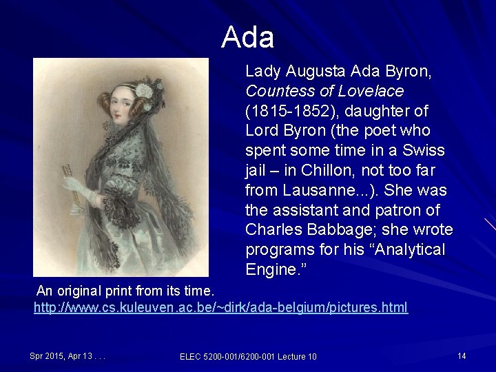
Ada Lady Augusta Ada Byron, Countess of Lovelace (1815 -1852), daughter of Lord Byron (the poet who spent some time in a Swiss jail – in Chillon, not too far from Lausanne. . . ). She was the assistant and patron of Charles Babbage; she wrote programs for his “Analytical Engine. ” An original print from its time. http: //www. cs. kuleuven. ac. be/~dirk/ada-belgium/pictures. html Spr 2015, Apr 13. . . ELEC 5200 -001/6200 -001 Lecture 10 14

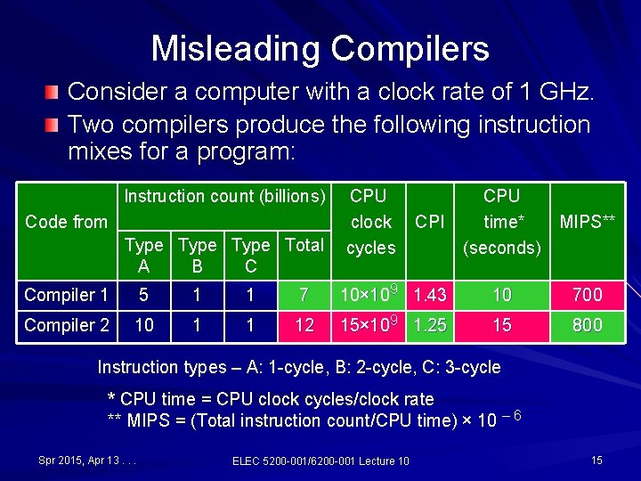
Misleading Compilers Consider a computer with a clock rate of 1 GHz. Two compilers produce the following instruction mixes for a program: Instruction count (billions) Code from Type Total A B C CPU clock cycles CPI CPU time* MIPS** (seconds) Compiler 1 5 1 1 7 10× 109 1. 43 10 700 Compiler 2 10 1 1 12 15× 109 1. 25 15 800 Instruction types – A: 1 -cycle, B: 2 -cycle, C: 3 -cycle * CPU time = CPU clock cycles/clock rate ** MIPS = (Total instruction count/CPU time) × 10 – 6 Spr 2015, Apr 13. . . ELEC 5200 -001/6200 -001 Lecture 10 15

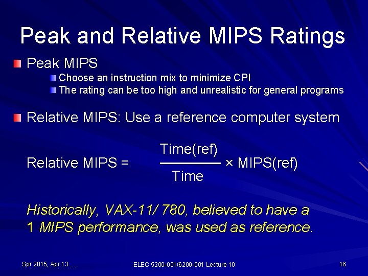
Peak and Relative MIPS Ratings Peak MIPS Choose an instruction mix to minimize CPI The rating can be too high and unrealistic for general programs Relative MIPS: Use a reference computer system Relative MIPS = Time(ref) ────── × MIPS(ref) Time Historically, VAX-11/ 780, believed to have a 1 MIPS performance, was used as reference. Spr 2015, Apr 13. . . ELEC 5200 -001/6200 -001 Lecture 10 16

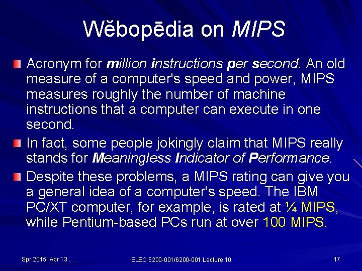
Wĕbopēdia on MIPS Acronym for million instructions per second. An old measure of a computer's speed and power, MIPS measures roughly the number of machine instructions that a computer can execute in one second. In fact, some people jokingly claim that MIPS really stands for Meaningless Indicator of Performance. Despite these problems, a MIPS rating can give you a general idea of a computer's speed. The IBM PC/XT computer, for example, is rated at ¼ MIPS, while Pentium-based PCs run at over 100 MIPS. Spr 2015, Apr 13. . . ELEC 5200 -001/6200 -001 Lecture 10 17

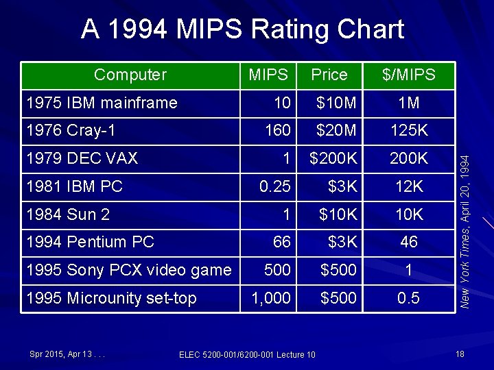
A 1994 MIPS Rating Chart MIPS 1975 IBM mainframe 1976 Cray-1 1979 DEC VAX 1981 IBM PC 1984 Sun 2 1994 Pentium PC 1995 Sony PCX video game 1995 Microunity set-top Spr 2015, Apr 13. . . Price $/MIPS 10 $10 M 1 M 160 $20 M 125 K 1 $200 K 0. 25 $3 K 12 K 1 $10 K 66 $3 K 46 500 $500 1 1, 000 $500 0. 5 ELEC 5200 -001/6200 -001 Lecture 10 New York Times, April 20, 1994 Computer 18

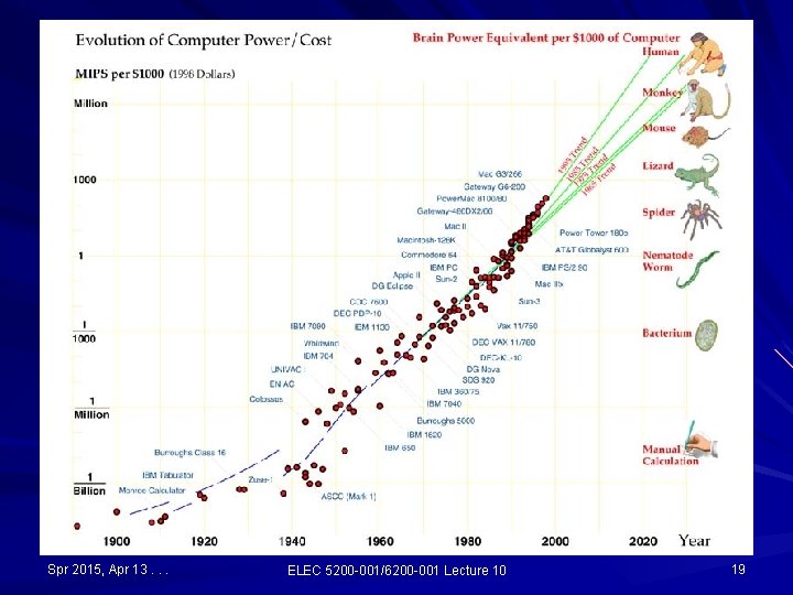
Spr 2015, Apr 13. . . ELEC 5200 -001/6200 -001 Lecture 10 19

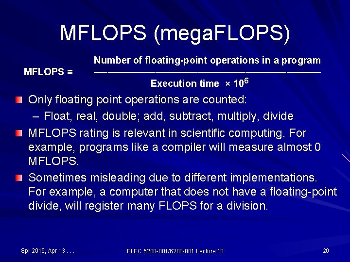
MFLOPS (mega. FLOPS) MFLOPS = Number of floating-point operations in a program ───────────────── Execution time × 106 Only floating point operations are counted: – Float, real, double; add, subtract, multiply, divide MFLOPS rating is relevant in scientific computing. For example, programs like a compiler will measure almost 0 MFLOPS. Sometimes misleading due to different implementations. For example, a computer that does not have a floating-point divide, will register many FLOPS for a division. Spr 2015, Apr 13. . . ELEC 5200 -001/6200 -001 Lecture 10 20

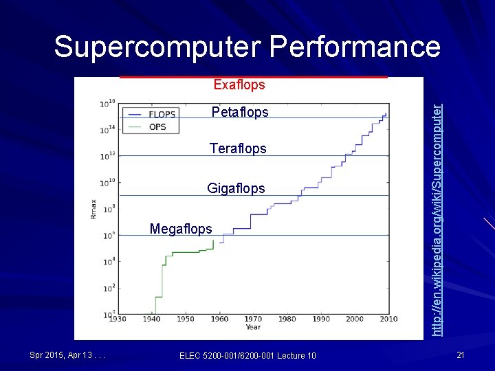
Supercomputer Performance Petaflops Teraflops Gigaflops Megaflops Spr 2015, Apr 13. . . ELEC 5200 -001/6200 -001 Lecture 10 http: //en. wikipedia. org/wiki/Supercomputer Exaflops 21

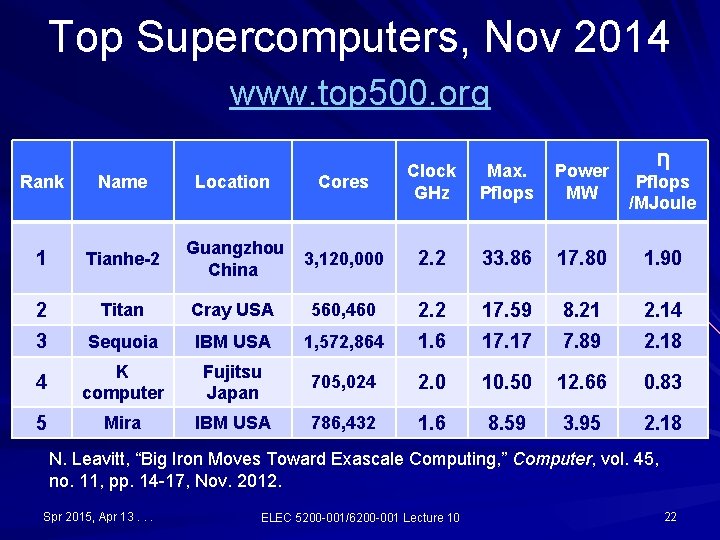
Top Supercomputers, Nov 2014 www. top 500. org Max. Pflops Power MW Ƞ Pflops /MJoule Rank Name Location Cores Clock GHz 1 Tianhe-2 Guangzhou China 3, 120, 000 2. 2 33. 86 17. 80 1. 90 2 Titan Cray USA 560, 460 2. 2 17. 59 8. 21 2. 14 3 Sequoia IBM USA 1, 572, 864 1. 6 17. 17 7. 89 2. 18 4 K computer Fujitsu Japan 705, 024 2. 0 10. 50 12. 66 0. 83 5 Mira IBM USA 786, 432 1. 6 8. 59 3. 95 2. 18 N. Leavitt, “Big Iron Moves Toward Exascale Computing, ” Computer, vol. 45, no. 11, pp. 14 -17, Nov. 2012. Spr 2015, Apr 13. . . ELEC 5200 -001/6200 -001 Lecture 10 22

The Future Erik P. De. Benedictis of Sandia National Laboratories theorizes that a zettaflops (1021) (one sextillion FLOPS) computer is required to accomplish full weather modeling, which could cover a two week time span accurately. Such systems might be built around 2030. http: //en. wikipedia. org/wiki/Supercomputer Spr 2015, Apr 13. . . ELEC 5200 -001/6200 -001 Lecture 10 23

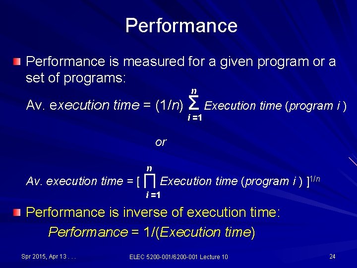
Performance is measured for a given program or a set of programs: n Av. execution time = (1/n) Σ Execution time (program i ) i =1 or n Av. execution time = [ ∏ Execution time (program i ) ]1/n i =1 Performance is inverse of execution time: Performance = 1/(Execution time) Spr 2015, Apr 13. . . ELEC 5200 -001/6200 -001 Lecture 10 24

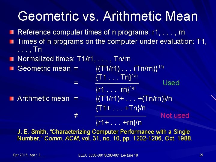
Geometric vs. Arithmetic Mean Reference computer times of n programs: r 1, . . . , rn Times of n programs on the computer under evaluation: T 1, . . . , Tn Normalized times: T 1/r 1, . . . , Tn/rn Geometric mean = {(T 1/r 1). . . (Tn/rn)}1/n {T 1. . . Tn}1/n = Used 1/n {r 1. . . rn} Arithmetic mean = {(T 1/r 1)+. . . +(Tn/rn)}/n {T 1+. . . +Tn}/n ≠ Not used {r 1+. . . +rn}/n J. E. Smith, “Characterizing Computer Performance with a Single Number, ” Comm. ACM, vol. 31, no. 10, pp. 1202 -1206, Oct. 1988. Spr 2015, Apr 13. . . ELEC 5200 -001/6200 -001 Lecture 10 25

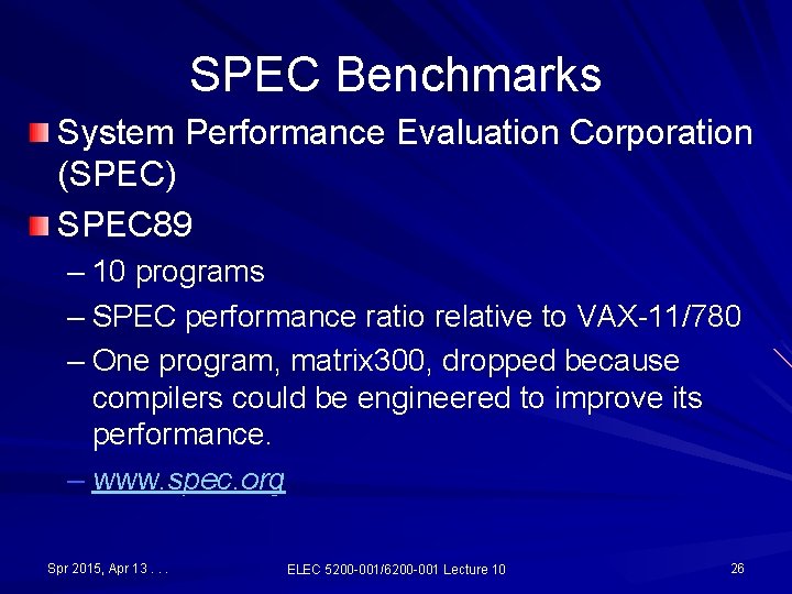
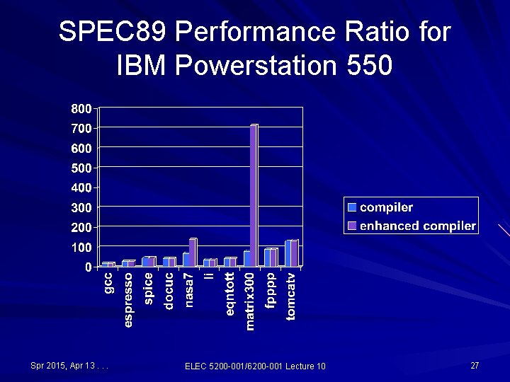
SPEC Benchmarks System Performance Evaluation Corporation (SPEC) SPEC 89 – 10 programs – SPEC performance ratio relative to VAX-11/780 – One program, matrix 300, dropped because compilers could be engineered to improve its performance. – www. spec. org Spr 2015, Apr 13. . . ELEC 5200 -001/6200 -001 Lecture 10 26

SPEC 89 Performance Ratio for IBM Powerstation 550 Spr 2015, Apr 13. . . ELEC 5200 -001/6200 -001 Lecture 10 27

SPEC 95 Benchmarks Eight integer and ten floating point programs, SPECint 95 and SPECfp 95. Each program run time is normalized with respect to the run time of Sun SPARCstation 10/40 – the ratio is called SPEC ratio. SPECint 95 and SPECfp 95 summary measurements are the geometric means of SPEC ratios. Spr 2015, Apr 13. . . ELEC 5200 -001/6200 -001 Lecture 10 28

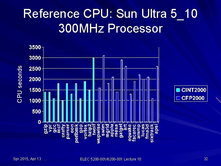
SPEC CPU 2000 Benchmarks Twelve integer and 14 floating point programs, CINT 2000 and CFP 2000. Each program run time is normalized to obtain a SPEC ratio with respect to the run time on Sun Ultra 5_10 with a 300 MHz processor. CINT 2000 and CFP 2000 summary measurements are the geometric means of SPEC ratios. Retired in 2007, replaced with SPEC CPUTM 2006 https: //www. spec. org/cpu 2006/ Spr 2015, Apr 13. . . ELEC 5200 -001/6200 -001 Lecture 10 29

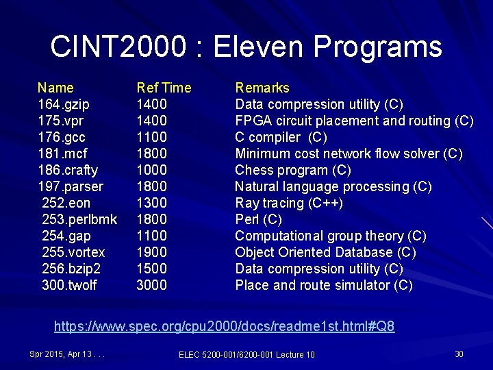
CINT 2000 : Eleven Programs Name 164. gzip 175. vpr 176. gcc 181. mcf 186. crafty 197. parser 252. eon 253. perlbmk 254. gap 255. vortex 256. bzip 2 300. twolf Ref Time 1400 1100 1800 1000 1800 1300 1800 1100 1900 1500 3000 Remarks Data compression utility (C) FPGA circuit placement and routing (C) C compiler (C) Minimum cost network flow solver (C) Chess program (C) Natural language processing (C) Ray tracing (C++) Perl (C) Computational group theory (C) Object Oriented Database (C) Data compression utility (C) Place and route simulator (C) https: //www. spec. org/cpu 2000/docs/readme 1 st. html#Q 8 Spr 2015, Apr 13. . . ELEC 5200 -001/6200 -001 Lecture 10 30

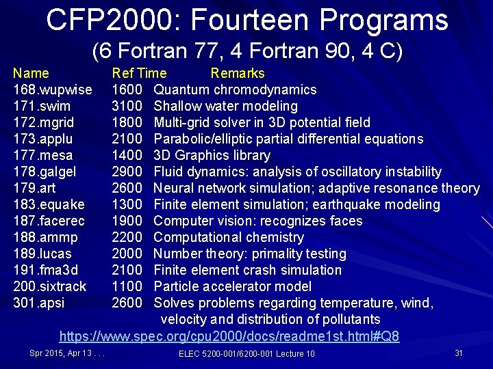
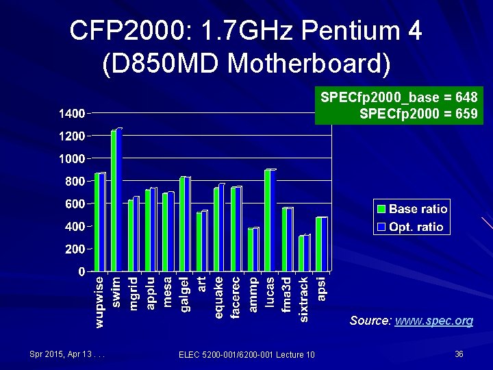
CFP 2000: Fourteen Programs (6 Fortran 77, 4 Fortran 90, 4 C) Name 168. wupwise 171. swim 172. mgrid 173. applu 177. mesa 178. galgel 179. art 183. equake 187. facerec 188. ammp 189. lucas 191. fma 3 d 200. sixtrack 301. apsi Ref Time Remarks 1600 Quantum chromodynamics 3100 Shallow water modeling 1800 Multi-grid solver in 3 D potential field 2100 Parabolic/elliptic partial differential equations 1400 3 D Graphics library 2900 Fluid dynamics: analysis of oscillatory instability 2600 Neural network simulation; adaptive resonance theory 1300 Finite element simulation; earthquake modeling 1900 Computer vision: recognizes faces 2200 Computational chemistry 2000 Number theory: primality testing 2100 Finite element crash simulation 1100 Particle accelerator model 2600 Solves problems regarding temperature, wind, velocity and distribution of pollutants https: //www. spec. org/cpu 2000/docs/readme 1 st. html#Q 8 Spr 2015, Apr 13. . . ELEC 5200 -001/6200 -001 Lecture 10 31

CPU seconds Reference CPU: Sun Ultra 5_10 300 MHz Processor Spr 2015, Apr 13. . . ELEC 5200 -001/6200 -001 Lecture 10 32

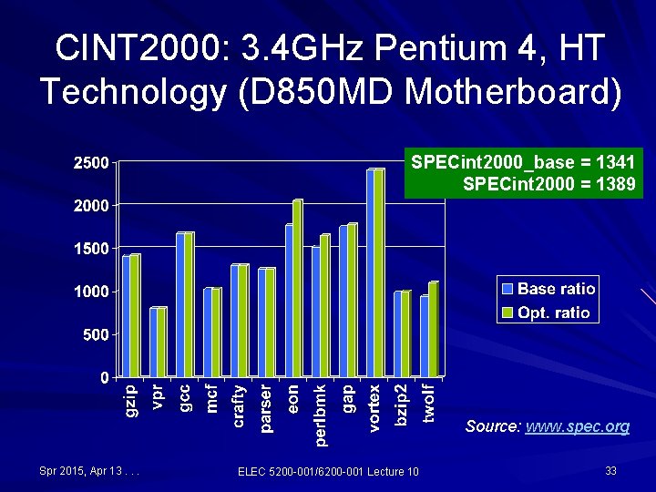
CINT 2000: 3. 4 GHz Pentium 4, HT Technology (D 850 MD Motherboard) SPECint 2000_base = 1341 SPECint 2000 = 1389 Source: www. spec. org Spr 2015, Apr 13. . . ELEC 5200 -001/6200 -001 Lecture 10 33

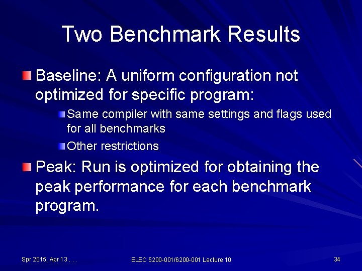
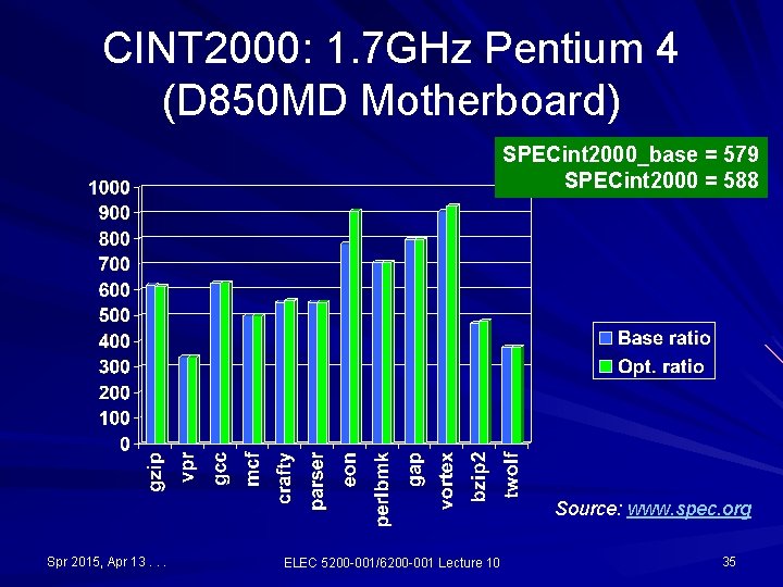
Two Benchmark Results Baseline: A uniform configuration not optimized for specific program: Same compiler with same settings and flags used for all benchmarks Other restrictions Peak: Run is optimized for obtaining the peak performance for each benchmark program. Spr 2015, Apr 13. . . ELEC 5200 -001/6200 -001 Lecture 10 34

CINT 2000: 1. 7 GHz Pentium 4 (D 850 MD Motherboard) SPECint 2000_base = 579 SPECint 2000 = 588 Source: www. spec. org Spr 2015, Apr 13. . . ELEC 5200 -001/6200 -001 Lecture 10 35

CFP 2000: 1. 7 GHz Pentium 4 (D 850 MD Motherboard) SPECfp 2000_base = 648 SPECfp 2000 = 659 Source: www. spec. org Spr 2015, Apr 13. . . ELEC 5200 -001/6200 -001 Lecture 10 36

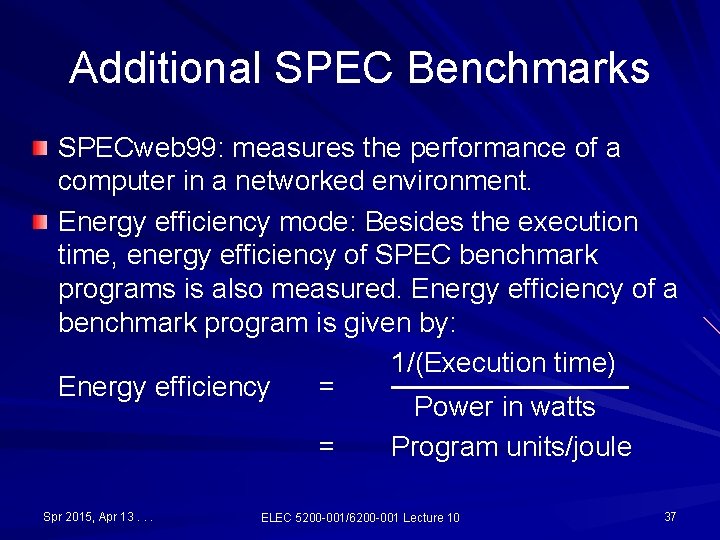
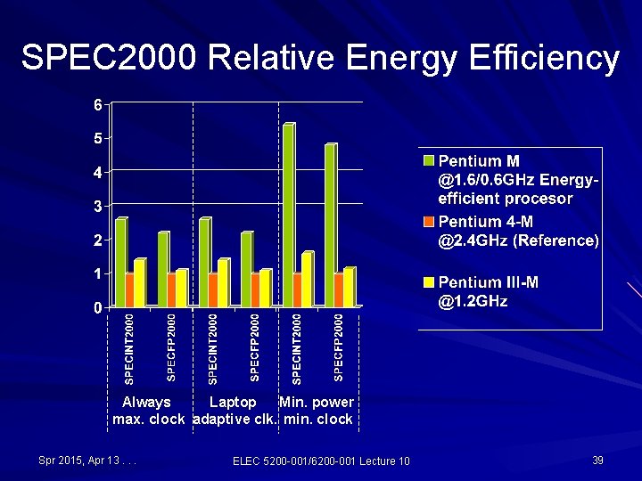
Additional SPEC Benchmarks SPECweb 99: measures the performance of a computer in a networked environment. Energy efficiency mode: Besides the execution time, energy efficiency of SPEC benchmark programs is also measured. Energy efficiency of a benchmark program is given by: 1/(Execution time) Energy efficiency = ────── Power in watts = Program units/joule Spr 2015, Apr 13. . . ELEC 5200 -001/6200 -001 Lecture 10 37

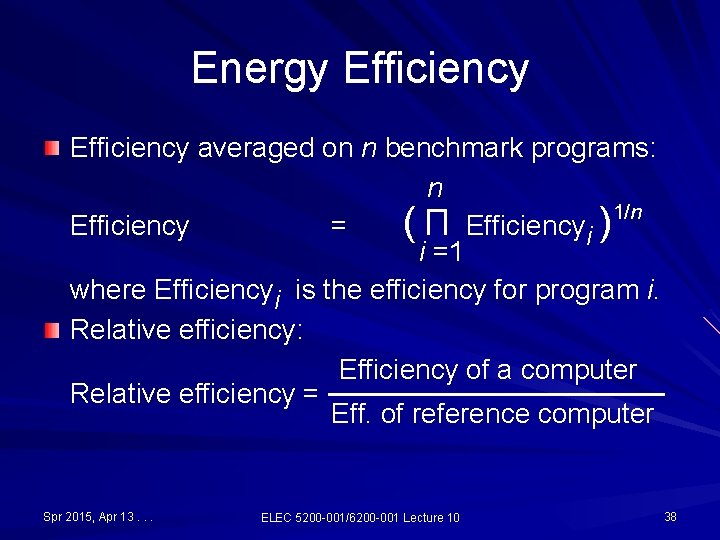
Energy Efficiency averaged on n benchmark programs: n 1/n Efficiency = ( Π Efficiencyi ) i =1 where Efficiencyi is the efficiency for program i. Relative efficiency: Efficiency of a computer Relative efficiency = ───────── Eff. of reference computer Spr 2015, Apr 13. . . ELEC 5200 -001/6200 -001 Lecture 10 38

SPEC 2000 Relative Energy Efficiency Always Laptop Min. power max. clock adaptive clk. min. clock Spr 2015, Apr 13. . . ELEC 5200 -001/6200 -001 Lecture 10 39

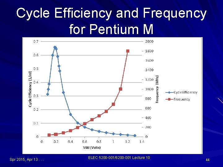
Energy and Time Perspectives Clock cycle is the unit of computing work. Cycle rate, f cycles per second f is the rate of doing computing work Hardware speed, similar to mph for a car Cycle efficiency, η cycles per joule η is the computing work per energy unit Hardware efficiency, similar to mpg for a car Results from recent work: – A. Shinde, “Managing Performance and Efficiency of a Processor, ” MEE Project Report, Auburn Univ. , Dec. 2012. – A. Shinde and V. D. Agarwal, “Managing Performance and Efficiency of a Processor, ” Proc. 45 th IEEE Southeastern Symposium on System Theory, Baylor Univ. , TX, March 2013, pp. 59 -62. Spr 2015, Apr 13. . . ELEC 5200 -001/6200 -001 Lecture 10 40

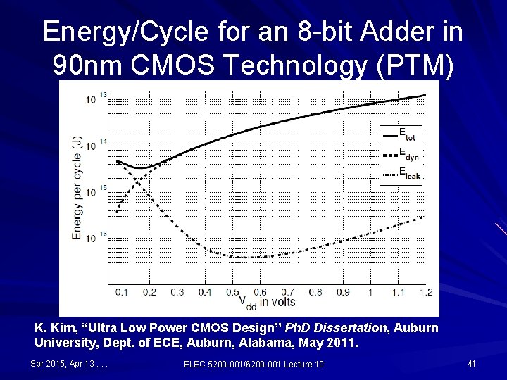
Energy/Cycle for an 8 -bit Adder in 90 nm CMOS Technology (PTM) K. Kim, “Ultra Low Power CMOS Design” Ph. D Dissertation, Auburn University, Dept. of ECE, Auburn, Alabama, May 2011. Spr 2015, Apr 13. . . ELEC 5200 -001/6200 -001 Lecture 10 41

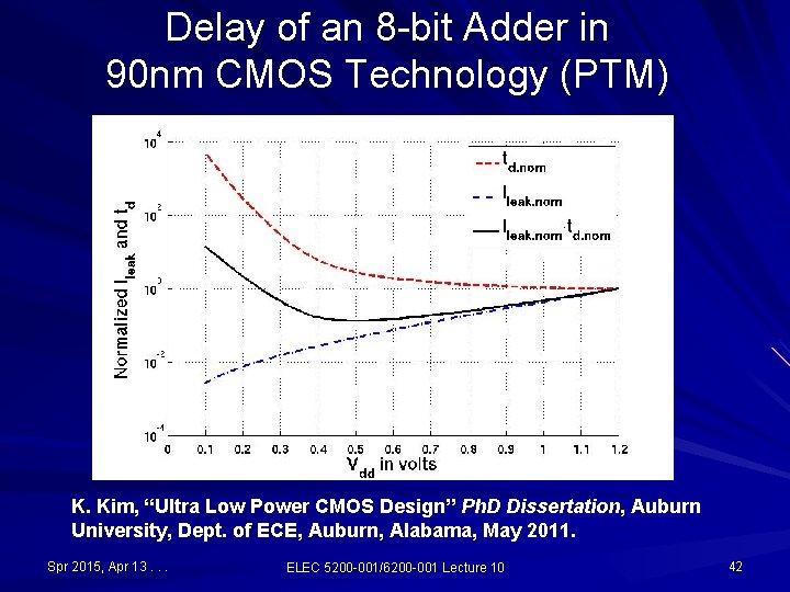
Delay of an 8 -bit Adder in 90 nm CMOS Technology (PTM) K. Kim, “Ultra Low Power CMOS Design” Ph. D Dissertation, Auburn University, Dept. of ECE, Auburn, Alabama, May 2011. Spr 2015, Apr 13. . . ELEC 5200 -001/6200 -001 Lecture 10 42

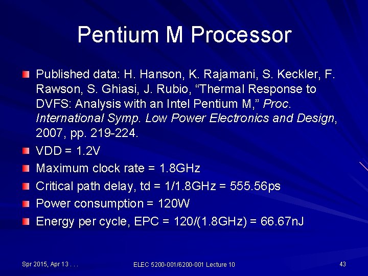
Pentium M Processor Published data: H. Hanson, K. Rajamani, S. Keckler, F. Rawson, S. Ghiasi, J. Rubio, “Thermal Response to DVFS: Analysis with an Intel Pentium M, ” Proc. International Symp. Low Power Electronics and Design, 2007, pp. 219 -224. VDD = 1. 2 V Maximum clock rate = 1. 8 GHz Critical path delay, td = 1/1. 8 GHz = 555. 56 ps Power consumption = 120 W Energy per cycle, EPC = 120/(1. 8 GHz) = 66. 67 n. J Spr 2015, Apr 13. . . ELEC 5200 -001/6200 -001 Lecture 10 43

Cycle Efficiency and Frequency for Pentium M Spr 2015, Apr 13. . . ELEC 5200 -001/6200 -001 Lecture 10 44

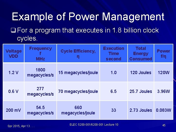
Example of Power Management q For a program that executes in 1. 8 billion clock cycles. Voltage VDD Frequency f MHz Cycle Efficiency, η Execution Time second Total Energy Consumed Power f/η 1. 2 V 1800 megacycles/s 15 megacycles/joule 1. 0 120 Joules 120 W 0. 6 V 277 megacycles/s 70 megacycles/joule 6. 5 25. 7 Joules 3. 96 W 200 m. V 54. 5 megacycles/s 660 megacycles/joule 33 2. 73 Joules 0. 083 W Spr 2015, Apr 13. . . ELEC 5200 -001/6200 -001 Lecture 10 45

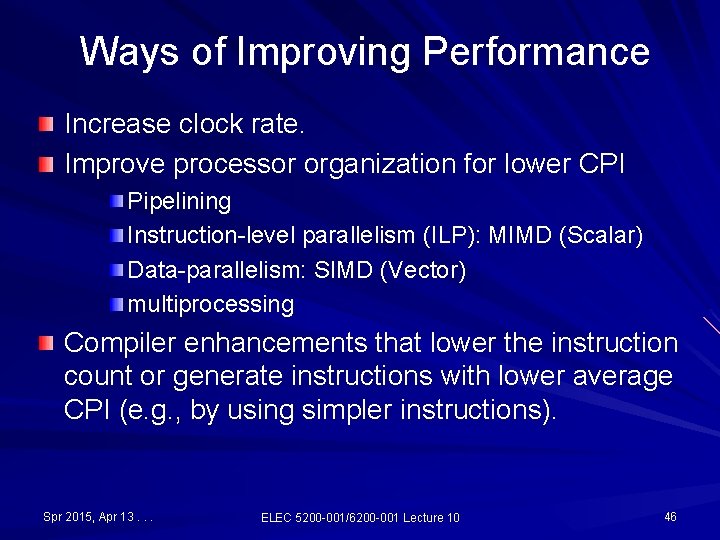
Ways of Improving Performance Increase clock rate. Improve processor organization for lower CPI Pipelining Instruction-level parallelism (ILP): MIMD (Scalar) Data-parallelism: SIMD (Vector) multiprocessing Compiler enhancements that lower the instruction count or generate instructions with lower average CPI (e. g. , by using simpler instructions). Spr 2015, Apr 13. . . ELEC 5200 -001/6200 -001 Lecture 10 46

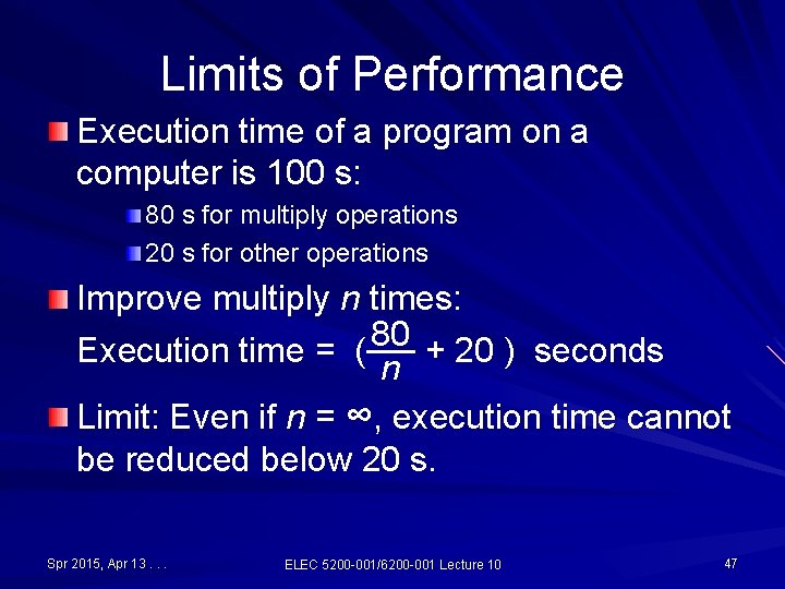
Limits of Performance Execution time of a program on a computer is 100 s: 80 s for multiply operations 20 s for other operations Improve multiply n times: 80 Execution time = (── n + 20 ) seconds Limit: Even if n = ∞, execution time cannot be reduced below 20 s. Spr 2015, Apr 13. . . ELEC 5200 -001/6200 -001 Lecture 10 47

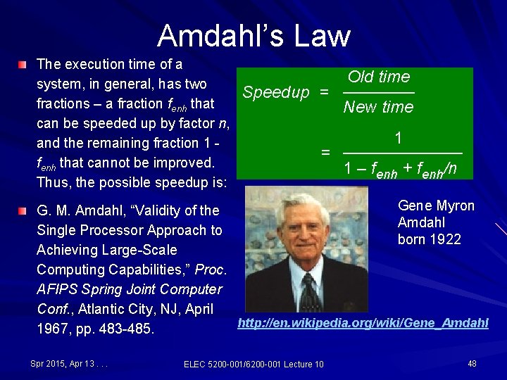
Amdahl’s Law The execution time of a system, in general, has two fractions – a fraction fenh that can be speeded up by factor n, and the remaining fraction 1 fenh that cannot be improved. Thus, the possible speedup is: Old time Speedup = ────── New time 1 = ───── 1 – fenh + fenh/n Gene Myron G. M. Amdahl, “Validity of the Amdahl Single Processor Approach to born 1922 Achieving Large-Scale Computing Capabilities, ” Proc. AFIPS Spring Joint Computer Conf. , Atlantic City, NJ, April http: //en. wikipedia. org/wiki/Gene_Amdahl 1967, pp. 483 -485. Spr 2015, Apr 13. . . ELEC 5200 -001/6200 -001 Lecture 10 48

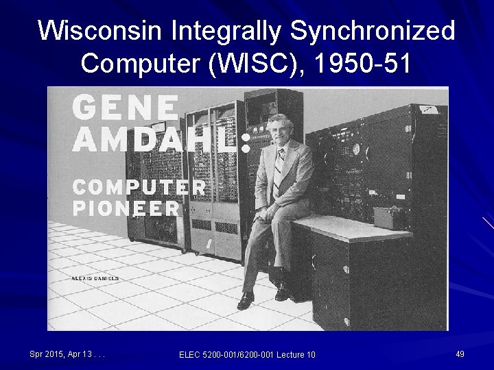
Wisconsin Integrally Synchronized Computer (WISC), 1950 -51 Spr 2015, Apr 13. . . ELEC 5200 -001/6200 -001 Lecture 10 49

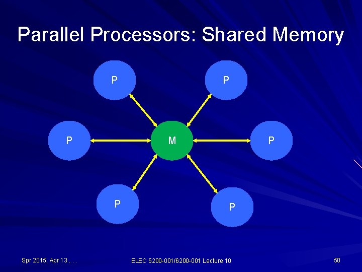
Parallel Processors: Shared Memory P P M P Spr 2015, Apr 13. . . P P P ELEC 5200 -001/6200 -001 Lecture 10 50

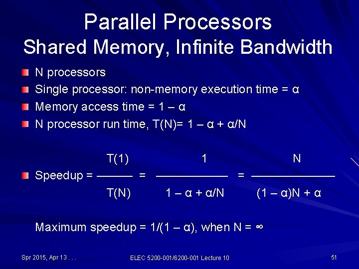
Parallel Processors Shared Memory, Infinite Bandwidth N processors Single processor: non-memory execution time = α Memory access time = 1 – α N processor run time, T(N)= 1 – α + α/N T(1) 1 N Speedup = ——————— T(N) 1 – α + α/N (1 – α)N + α Maximum speedup = 1/(1 – α), when N = ∞ Spr 2015, Apr 13. . . ELEC 5200 -001/6200 -001 Lecture 10 51

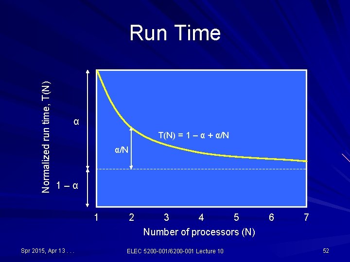
Normalized run time, T(N) Run Time α T(N) = 1 – α + α/N 1–α 1 Spr 2015, Apr 13. . . 2 3 4 5 Number of processors (N) ELEC 5200 -001/6200 -001 Lecture 10 6 7 52

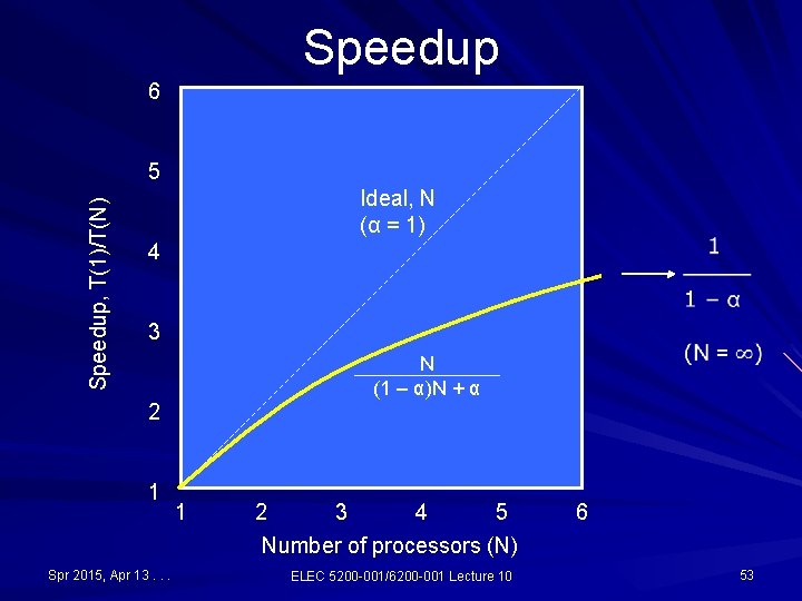
Speedup 6 Speedup, T(1)/T(N) 5 Ideal, N (α = 1) 4 3 N (1 – α)N + α 2 1 Spr 2015, Apr 13. . . 1 2 3 4 5 Number of processors (N) ELEC 5200 -001/6200 -001 Lecture 10 6 53

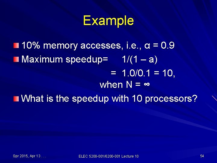
Example 10% memory accesses, i. e. , α = 0. 9 Maximum speedup= 1/(1 – a) = 1. 0/0. 1 = 10, when N = ∞ What is the speedup with 10 processors? Spr 2015, Apr 13. . . ELEC 5200 -001/6200 -001 Lecture 10 54

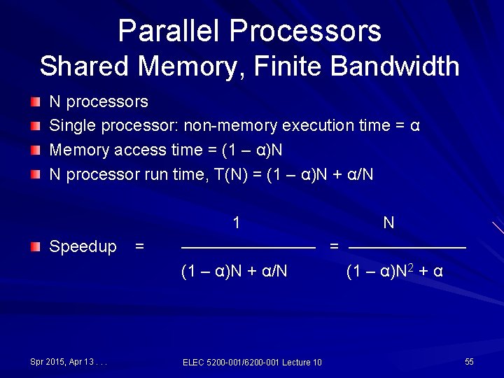
Parallel Processors Shared Memory, Finite Bandwidth N processors Single processor: non-memory execution time = α Memory access time = (1 – α)N N processor run time, T(N) = (1 – α)N + α/N Speedup Spr 2015, Apr 13. . . = 1 N ———— = ——————— (1 – α)N + α/N (1 – α)N 2 + α ELEC 5200 -001/6200 -001 Lecture 10 55

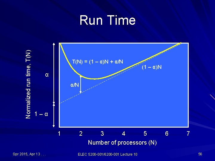
Normalized run time, T(N) Run Time T(N) = (1 – α)N + α/N (1 – α)N α α/N 1–α 1 Spr 2015, Apr 13. . . 2 3 4 5 Number of processors (N) ELEC 5200 -001/6200 -001 Lecture 10 6 7 56

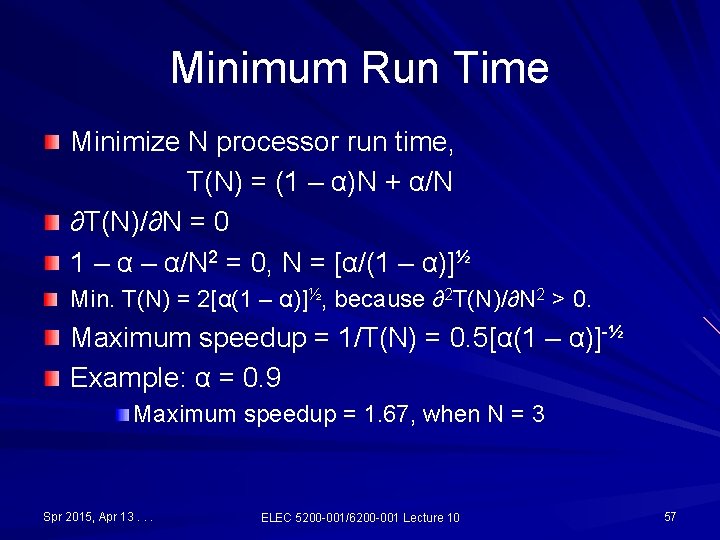
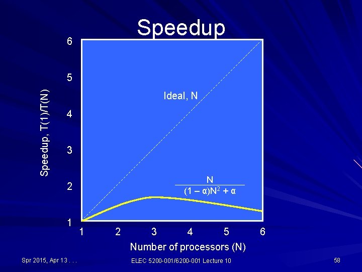
Minimum Run Time Minimize N processor run time, T(N) = (1 – α)N + α/N ∂T(N)/∂N = 0 1 – α/N 2 = 0, N = [α/(1 – α)]½ Min. T(N) = 2[α(1 – α)]½, because ∂2 T(N)/∂N 2 > 0. Maximum speedup = 1/T(N) = 0. 5[α(1 – α)]-½ Example: α = 0. 9 Maximum speedup = 1. 67, when N = 3 Spr 2015, Apr 13. . . ELEC 5200 -001/6200 -001 Lecture 10 57

Speedup 6 Speedup, T(1)/T(N) 5 Ideal, N 4 3 N (1 – α)N 2 + α 2 1 Spr 2015, Apr 13. . . 1 2 3 4 5 Number of processors (N) ELEC 5200 -001/6200 -001 Lecture 10 6 58

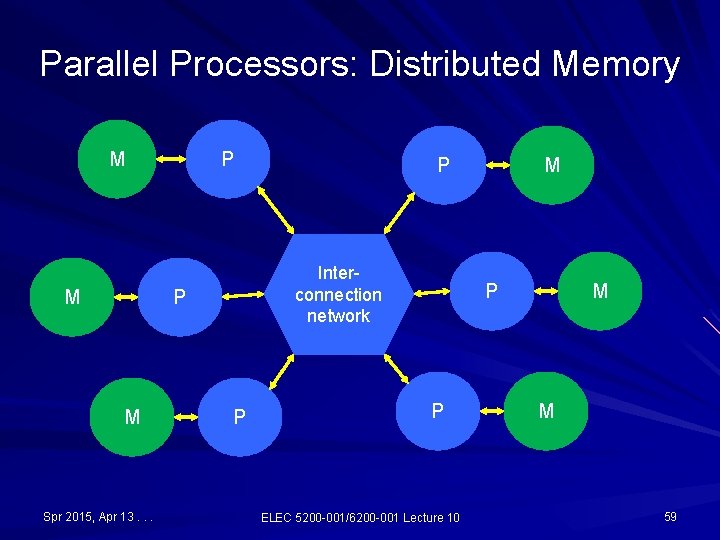
Parallel Processors: Distributed Memory M M P Interconnection network P M Spr 2015, Apr 13. . . P P M P P ELEC 5200 -001/6200 -001 Lecture 10 M M 59

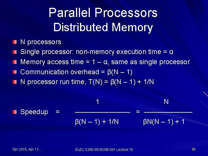
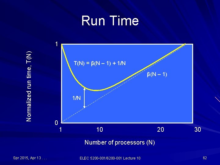
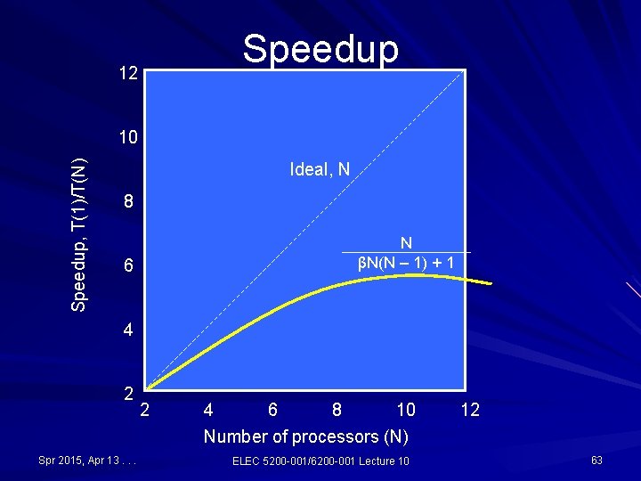
Parallel Processors Distributed Memory N processors Single processor: non-memory execution time = α Memory access time = 1 – α, same as single processor Communication overhead = β(N – 1) N processor run time, T(N) = β(N – 1) + 1/N Speedup Spr 2015, Apr 13. . . = 1 N ———— = ——————— β(N – 1) + 1/N βN(N – 1) + 1 ELEC 5200 -001/6200 -001 Lecture 10 60

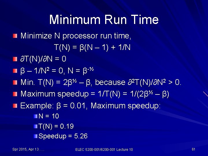
Minimum Run Time Minimize N processor run time, T(N) = β(N – 1) + 1/N ∂T(N)/∂N = 0 β – 1/N 2 = 0, N = β-½ Min. T(N) = 2β½ – β, because ∂2 T(N)/∂N 2 > 0. Maximum speedup = 1/T(N) = 1/(2β½ – β) Example: β = 0. 01, Maximum speedup: N = 10 T(N) = 0. 19 Speedup = 5. 26 Spr 2015, Apr 13. . . ELEC 5200 -001/6200 -001 Lecture 10 61

Run Time Normalized run time, T(N) 1 T(N) = β(N – 1) + 1/N β(N – 1) 1/N 0 1 10 20 30 Number of processors (N) Spr 2015, Apr 13. . . ELEC 5200 -001/6200 -001 Lecture 10 62

Speedup 12 Speedup, T(1)/T(N) 10 Ideal, N 8 N βN(N – 1) + 1 6 4 2 Spr 2015, Apr 13. . . 2 4 6 8 10 Number of processors (N) ELEC 5200 -001/6200 -001 Lecture 10 12 63

Further Reading G. M. Amdahl, “Validity of the Single Processor Approach to Achieving Large- G. M. Amdahl, “Validity of the Single Processor Approach to Achieving Large. Scale Computing Capabilities, ” Proc. AFIPS Spring Joint Computer Conf. , Atlantic City, NJ, Apr. 1967, pp. 483 -485. J. L. Gustafson, “Reevaluating Amdahl’s Law, ” Comm. ACM, vol. 31, no. 5, pp. 532 -533, May 1988. M. D. Hill and M. R. Marty, “Amdahl’s Law in the Multicore Era, ” Computer, vol. 41, no. 7, pp. 33 -38, July 2008. D. H. Woo and H. -H. S. Lee, “Extending Amdahl’s Law for Energy-Efficient Computing in the Many-Core Era, ” Computer, vol. 41, no. 12, pp. 24 -31, Dec. 2008. S. M. Pieper, J. M. Paul and M. J. Schulte, “A New Era of Performance Evaluation, ” Computer, vol. 40, no. 9, pp. 23 -30, Sep. 2007. S. Gal-On and M. Levy, “Measuring Multicore Performance, ” Computer, vol. 41, no. 11, pp. 99 -102, November 2008. S. Williams, A. Waterman and D. Patterson, “Roofline: An Insightful Visual Performance Model for Multicore Architectures, ” Comm. ACM, vol. 52, no. 4, pp. 65 -76, Apr. 2009. U. Vishkin, “Is Multicore Hardware for General-Purpose Parallel Processing Broken? ” Comm. ACM, vol. 57, no. 4, pp. 35 -39, Apr. 2014. Spr 2015, Apr 13. . . ELEC 5200 -001/6200 -001 Lecture 10 64