Digital and NonLinear Control Root Locus Outline Introduction

Digital and Non-Linear Control Root Locus

Outline • • Introduction Angle and Magnitude Condition Construction of Root Loci Examples

Introduction • Consider a unity feedback control system shown below. • The open loop transfer function G(s) of the system is • And the closed transfer function is

Introduction • Location of closed loop Pole for different values of K (remember K>0). K 0. 5 1 2 Pole -1. 5 -2 -3 3 5 10 15 -4 -6 -11 -16

What is Root Locus? • The root locus is the path of the roots of the characteristic equation traced out in the s-plane as a system parameter varies from zero to infinity.

How to Sketch root locus? • One way is to compute the roots of the characteristic equation for all possible values of K. K 0. 5 1 2 Pole -1. 5 -2 -3 3 5 10 15 -4 -6 -11 -16

How to Sketch root locus? • Computing the roots for all values of K might be tedious for higher order systems. K 0. 5 1 2 Pole ? ? ? 3 5 10 15 ? ?

Construction of Root Loci • Finding the roots of the characteristic equation of degree higher than 3 is laborious and will need computer solution. • A simple method for finding the roots of the characteristic equation has been developed by W. R. Evans and used extensively in control engineering. • This method, called the root-locus method, is one in which the roots of the characteristic equation are plotted for all values of a system parameter.

Construction of Root Loci • The roots corresponding to a particular value of this parameter can then be located on the resulting graph. • By using the root-locus method the designer can predict the effects on the location of the closed-loop poles of varying the gain value or adding open-loop poles and/or open-loop zeros.

Angle & Magnitude Conditions • In constructing the root loci angle and magnitude conditions are important. • Consider the system shown in following figure. • The closed loop transfer function is

Construction of Root Loci • The characteristic equation is obtained by setting the denominator polynomial equal to zero. • Or • Since G(s)H(s) is a complex quantity it can be split into angle and magnitude part.

Angle & Magnitude Conditions • The angle of G(s)H(s)=-1 is • Where k=1, 2, 3… • The magnitude of G(s)H(s)=-1 is

Angle & Magnitude Conditions • Angle Condition • Magnitude Condition • The values of s that fulfill both the angle and magnitude conditions are the roots of the characteristic equation, or the closed-loop poles.

Construction of root loci • Step-1: The first step in constructing a root-locus plot is to locate the open-loop poles and zeros in s-plane.

Construction of root loci • Step-2: Determine the root loci on the real axis. • To determine the root loci on real axis we select some test points. • e. g: p 1 (on positive real axis). p 1 • The angle condition is not satisfied. • Hence, there is no root locus on the positive real axis.

Construction of root loci • Step-2: Determine the root loci on the real axis. • Next, select a test point on the negative real axis between 0 and – 1. • Then • Thus • The angle condition is satisfied. Therefore, the portion of the negative real axis between 0 and – 1 forms a portion of the root locus. p 2

Construction of root loci • Step-2: Determine the root loci on the real axis. • Now, select a test point on the negative real axis between -1 and – 2. • Then • Thus • The angle condition is not satisfied. Therefore, the negative real axis between -1 and – 2 is not a part of the root locus. p 3

Construction of root loci • Step-2: Determine the root loci on the real axis. • Similarly, test point on the negative real axis between -2 and – ∞ satisfies the angle condition. p 4 • Therefore, the negative real axis between -2 and – ∞ is part of the root locus.

Construction of root loci • Step-2: Determine the root loci on the real axis.

Construction of root loci • Step-3: Determine the asymptotes of the root loci. That is, the root loci when s is far away from origin. Asymptote is the straight line approximation of a curve Actual Curve Asymptotic Approximation

Construction of root loci • Step-3: Determine the asymptotes of the root loci. • where • n-----> number of poles • m-----> number of zeros • For this Transfer Function

Construction of root loci • Step-3: Determine the asymptotes of the root loci. • Since the angle repeats itself as k is varied, the distinct angles for the asymptotes are determined as 60°, – 60°, and 180°.

Construction of root loci • Step-3: Determine the asymptotes of the root loci. • Before we can draw these asymptotes in the complex plane, we need to find the point where they intersect the real axis. • Point of intersection of asymptotes on real axis (or centroid of asymptotes) is

Construction of root loci • Step-3: Determine the asymptotes of the root loci. • For

Construction of root loci • Step-3: Determine the asymptotes of the root loci.

Construction of root loci • Step-4: Determine the breakaway/break-in point. • The breakaway/break-in point is the point from which the root locus branches leaves/arrives real axis.

Construction of root loci • Step-4: Determine the breakaway point or break-in point. • The breakaway or break-in points can be determined from the roots of (page 275) • It should be noted that not all the solutions of d. K/ds=0 correspond to actual breakaway points. • If a point at which d. K/ds=0 is on a root locus, it is an actual breakaway or break-in point.

Construction of root loci • Step-4: Determine the breakaway point or break-in point. • The characteristic equation of the system is • The breakaway point can now be determined as

Construction of root loci • Step-4: Determine the breakaway point or break-in point. • Set d. K/ds=0 in order to determine breakaway point.

Construction of root loci • Step-4: Determine the breakaway point or break-in point. • Since the breakaway point needs to be on a root locus between 0 and – 1, it is clear that s=– 0. 4226 corresponds to the actual breakaway point. • Point s=– 1. 5774 is not on the root locus. Hence, this point is not an actual breakaway or break-in point.

Construction of root loci • Step-4: Determine the breakaway point.

Construction of root loci • Step-4: Determine the breakaway point.

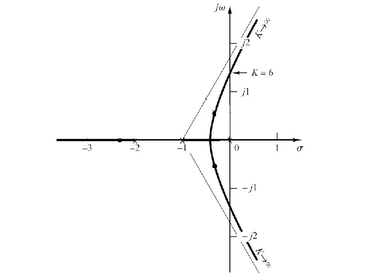
Construction of root loci • Step-5: Determine the points where root loci cross the imaginary axis.

Construction of root loci • Step-5: Determine the points where root loci cross the imaginary axis. • Let s=jω in the characteristic equation, equate both the real part and the imaginary part to zero, and then solve for ω and K. • For present system the characteristic equation is

Construction of root loci • Step-5: Determine the points where root loci cross the imaginary axis. • Equating both real and imaginary parts of this equation to zero • Which yields

Example • Determine the Breakaway and breakin points

Solution • Differentiating K with respect to s and setting the derivative equal to zero yields; Hence, solving for s, we find the break-away and break-in points s = -1. 45 and 3. 82

Solution -1. 45 3. 82

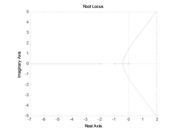
Root Loci by MATLAB • Example 6 -4 in page 293