Chapter 9 Design via Root Locus Improving transient

Chapter 9 Design via Root Locus

Improving transient response Figure 9. 1 a. Sample root locus, showing possible design point via gain adjustment (A) and desired design point that cannot be met via simple gain adjustment (B); b. responses from poles at A and B

Improving steady-state error Compensation techniques: a. cascade; b. feedback Ideal compensators are implemented with active networks.

Improving steady-state error via cascade compensation Pole at A is: a. on the root locus without compensator; b. not on the root locus with compensator pole added; (figure continues)

Ideal Integral compensation (PI) c. approximately on the root locus with compensator pole and zero added

Closed-loop system for Example 9. 1 a. before compensation; b. after ideal integral compensation Problem: The given system operating with damping ratio of 0. 174. Add an ideal integral compensator to reduce the ss error. Solution: We compensate the system by choosing a pole at the origin and a zero at -0. 1

Root locus for uncompensated system of Figure 9. 4(a) The gain K = 164. 6 yields Kp= 8. 23 and

Root locus for compensated system of Figure 9. 4(b) Almost same transient response and gain, but with zero ss error since we have a type one system.

Ideal integral compensated system response and the uncompensated system response of Example 9. 1

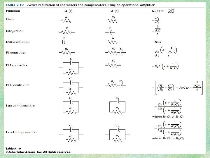
PI controller A method to implement an Ideal integral compensator is shown.

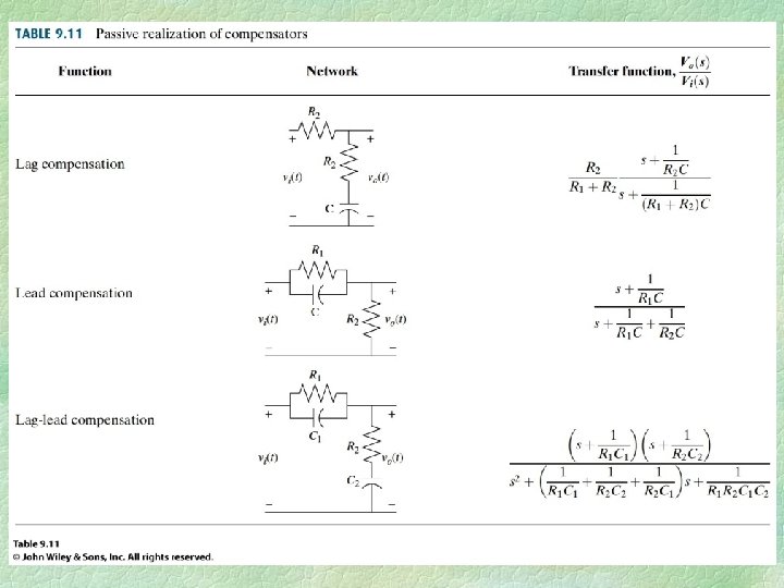
Lag Compensator a. Type 1 uncompensated system; b. Type 1 compensated system; c. compensator pole-zero plot Using passive networks, the compensation pole and zero is moved to the left, close to the origin. The static error constant for uncompensated system is Assuming the compensator is used as in b & c the static error is

Effect on transient response Root locus: a. before lag compensation; b. after lag compensation Almost no change on the transient response and same gain K. While the ss error is effected since

Lag compensator design Example 9. 2 Problem: Compensate the shown system to improve the ss error by a factor of 10 if the system is operating with a damping ratio of 0. 174 Solution: the uncompensated system error from previous example is 0. 108 with Kp= 8. 23. a ten fold improvement means ss error = 0. 0108 so Kp= 91. 59. so the ratio arbitrarily selecting Pc=0. 01 and Zc=11. 13 Pc 0. 111

Root locus for compensated system

Predicted characteristics of uncompensated and lag-compensated systems for Example 9. 2

Step responses of uncompensated and lag-compensated systems for Example 9. 2

Step responses of the system for Example 9. 2 using different lag compensators

Improving Transient response via Cascade Compensation Ideal Derivative compensator is called PD controller When using passive network it’s called lead compensator Using ideal derivative compensation: a. uncompensated; b. compensator zero at – 2;

Improving Transient response via Cascade Compensation c. Compensator zero at – 3; d. Compensator zero at – 4

Uncompensated system and ideal derivative compensation solutions from Table 9. 2

Table 9. 2 Predicted characteristics for the systems of previous slides

Feedback control system for Example 9. 3 Problem: Given the system in the figure, design an ideal derivative compensator to yield a 16% overshoot with a threefold reduction in settling time. Root locus for uncompensated system of Example 9. 3

Compensated dominant pole superimposed over the uncompensated root locus for Example 9. 3 The settling time for the uncompensated system shown in next slide is In order to have a threefold reduction in the settling time, the settling time of the compensated system will be one third of 3. 32 that is 1. 107, so the real part of the compensated system’s dominant second order pole is And the imaginary part is The figure shows the designed dominant 2 nd order poles.

Evaluating the location of the compensating zero for Example 9. 3 The sum of angles from all poles to the desired compensated pole 3. 613+j 6. 193 is -275. 6 The angle of the zero to be on the root locus is 275. 6 -180=95. 6 The location of the compensator zero is calculated as

Uncompensated and compensated system characteristics for Example 9. 3

Root locus for the compensated system of Example 9. 3

Uncompensated and compensated system step responses of Example 9. 3

PD controller implementation K 2 is chosen to contribute to the required loop-gain value. And K 1/K 2 is chosen to equal the negative of the compensator zero.

Geometry of lead compensation Advantages of a passive lead network over an active PD controller: 1) no need for additional power supply 2) noise due to differentiation is reduced Three of the infinite possible lead compensator solutions

Lead compensator design, Example 9. 4 Problem: Design 3 lead compensators for the system in figure that will reduce the settling time by a factor of 2 while maintaining 30% overshoot. Solution: The uncompensated settling time is To find the design point, new settling time is From which the real part of the desired pole location is And the imaginary part is

S-plane picture used to calculate the location of the compensator pole for Example 9. 4 Arbitrarily assume a compensator zero at -5 on the real axis as possible solution. Then we find the compensator pole location as shown in figure. Note sum of angles of compensator zero and all uncompensated poles and zeros is -172, 69 so the angular contribution of the compensator pole is -7. 31.

Compensated system root locus

Comparison of lead compensation designs for Example 9. 4

Uncompensated system and lead compensation responses for Example 9. 4

Improving Steady-State Error and Transient Response PID controller or using passive network it’s called lag-lad compensator

PID controller design Design Steps: v v v v Evaluate the performance of the uncompensated system to determine how much improvement is required in transient response Design the PD controller to meet the transient response specifications. The design includes the zero location and the loop gain. Simulate the system to be sure all requirements have been met. Redesign if the simulation shows that requirements have not been met. Design the PI controller to yield the required steady-sate error. Determine the gains, K 1, K 2, and K 3 shown in previous figure. Simulate the system to be sure all requirements have been met. Redesign if simulation shows that requirements have not been met.

PID controller design Example 9. 5 Problem: Using the system in the Figure, Design a PID controller so that the system can operate with a peak time that is 2/3 that of the uncompensated system at 20% overshoot and with zero steady-state error for a step input Solution: The uncompensated system operating at 20% overshoot has dominant poles at -5. 415+j 10. 57 with gain 121. 5, and a third pole at -8. 169. The complete performance is shown in next table.

Root locus for the uncompensated system of Example 9. 5 To compensate the system to reduce the peak time to 2/3 of original, we must find the compensated system dominant pole location. The imaginary part of the dominant pole is Thus the real part is

Predicted characteristics of uncompensated, PD- , and PIDcompensated systems of Example 9. 5

Calculating the PD compensator zero for Example 9. 5 To design the compensator, we find the sum of angles from the uncompensated system’s poles and zeros to the desired compensated dominant pole to be -198. 37. Thus the contribution required from the compensator zero is 198. 37 -180=18. 37. Then we calculate the location of the zero as: Thus the PD controller is GPD(s) = (s+55. 92) The complete root locus sketch is shown in next slide. Using program the gain at the design point is 5. 34

Root locus for PD-compensated system of Example 9. 5

Step responses for uncompensated, PD-compensated, and PIDcompensated systems of Example 9. 5

Root locus for PID-compensated system of Example 9. 5 Choosing the ideal integral compensator to be And sketching the root locus for the PID-compensated system as shown. Searching the 0. 456 damping ratio line, we find the dominant poles at -7. 516+j 14. 67 The characteristics of the PID compensated system are shown in table.

Predicted characteristics of uncompensated, PD- , and PIDcompensated systems of Example 9. 5

Improving Steady-State Error and Transient Response Finally to implement the compensator and find the K’s, using the PD and PI compensators and compare to we find K 1= 259. 5, K 2=128. 6, and K 3=4. 6

Lag-Lead Compensator Design Example 9. 6 Problem: Using the system in the Figure, Design a lag-lead compensator so that the system can operate with a twofold reduction in settling time, and 20% overshoot and a tenfold improvement in steady-state error for a ramp input Solution: The uncompensated system operating at 20% overshoot has dominant poles at -1. 794+j 3. 501 with gain 192. 1, and a third pole at -12. 41. The complete performance is shown in next table.

Root locus for uncompensated system of Example 9. 6 To compensate the system to realize a twofold reduction in settling time, the real part of the dominant poles must be increased by a factor of 2, thus, And the imaginary part is

Predicted characteristics of uncompensated, lead-compensated, and lag-lead- compensated systems of Example 9. 6

Evaluating the compensator pole for Example 9. 6 Now to design the lead compensator, arbitrarily select a location for the lead compensator zero at -6, to cancel the pole. To find the location of the compensator pole. Using program sum the angles to get -164. 65. and the contribution of the pole is -15. 35 we find the location of the pole from the figure as Results are satisfactory see results in next slide

Root locus for lead-compensated system of Example 9. 6

Improvement in step response for lag-lead- compensated system of Example 9. 6

Root locus for lag-lead- compensated system of Example 9. 6 Since the uncompensated system’s open-loop transfer function is The static error constant of the uncompensated system is 3. 201 Since the open-loop transfer function of the lead-compensated system is the static error constant of the lead-compensated system is 6. 794, so we have improvement by a factor of 2. 122. To improve the original system error by a factor of 10, the lag compensator must be designed to improve the error by a factor of 10/2. 122 = 4. 713

Root locus for lag-lead- compensated system of Example 9. 6 We arbitrarily choose the lag compensator pole at 0. 01, which then places the zero at 0. 04713 yielding as a lag compensator and as lag-lead-compensated system openloop transfer function

Predicted characteristics of uncompensated, lead-compensated, and lag-lead- compensated systems of Example 9. 6

Improvement in step response for lag-lead- compensated system of Example 9. 6

Improvement in ramp response error for the system of Example 9. 6:

a. Root locus before cascading notch filter; b. typical closed-loop step response before cascading notch filter; c. pole-zero plot of a notch filter; d. root locus after cascading notch filter; e. closed-loop step response after cascading notch filter.

Types of cascade compensators

Types of cascade compensators

Generic control system with feedback compensation Equivalent block diagram

a. Transfer function of a tachometer b. Tachometer feed-back compensation

Equivalent block diagram for the feedback compensator The Figure shows that the loop gain, G(s)H(s), is G(s)H(s) = K 1 G 1(s){Kf. Hc(s)+KG 2(s)} Without feedback, Kf. Hc(s), the loop gain is G(s)H(s) = KK 1 G 1(s)G 2(s) Thus, the effect of adding feedback is to replace the poles and zeros of G 2(s) with the poles and zeros of [Kf. Hc(s) + KG 2(s)]. Hence, this method is similar to cascade compensation in that we add new poles and zeros via H(s) to reshape the root locus to go through the design point. However, one must remember that zeros of the equivalent feedback shown in the Figure, H(s) = [Kf. Hc(s) +KG 2(s)]/KG 2(s), are not closed-loop zeros. For example, if G 2(s) = 1 and the minor-loop feedback, Kf. Hc(s), is a rate sensor, = Kf. S, then the loop gain is G(s)H(s) = Kf. K 1 G 1(s)(s+K/Kf) Thus, a zero at -K/Kf is added to the existing open-loop poles and zeros. This zero reshapes the root locus to go through the desired design point. Again, this zero is not a closed-loop zero.

Example 9. 7 Compensating Zero via Rate Feedback PROBLEM: Given the system of Figure 9. 49(a), design rate feedback compensation, as shown in Figure 9. 49(b), to reduce the settling time by a factor of 4 while continuing to operate the system with 20% overshoot. SOLUTION: First design a PD compensator. For the uncompensated system, search along the 20% overshoot line (ξ = 0. 456) and find that the dominant poles are at -1. 809 ±j 3. 531, as shown in Figure in next slide.

Root locus for uncompensated system The settling time is 2. 21 seconds and must be reduced by a factor of 4 to 0. 55 second. Next determine the location of the dominant poles for the compensated system. To achieve a fourfold decrease in the settling time, the real part of the pole must be increased by a factor of 4. Thus, the compensated pole has a real part of 4(-1. 809) = -7. 236. The imaginary part is then ωd = -7. 236 tan 117. 13° = 14. 12 where 117. 13° is the angle of the 20% overshoot line.

Step response for uncompensated system of Example

Predicted characteristics of uncompensated and compensated systems of Example

Finding the compensator zero in Example Using the compensated dominant pole position of -7. 236 ±j 14. 12, we sum the angles from the uncompensated system's poles and obtain 277. 33°. This angle requires a compensator zero contribution of +97. 33° to yield 180° at the design point. The geometry shown in the Figure leads to the calculation of the compensator's zero location. Hence, 14. 12/ (7. 236 – zc) = tan(180° - 97. 33°); from which zc = 5. 42.

Root locus for the compensated system of Example The root locus for the equivalent compensated system is shown in the Figure. The gain at the design point, which is K 1 Kf from Figure 9. 49(c), is found to be 256. 7. Since Kf is the reciprocal of the compensator zero, Kf = 0. 185. Thus, K 1 = 1388. In order to evaluate the steady-state error characteristic, Kv is found from Figure 9. 49(d) to be Kv = K 1 /(75 + K 1 Kf) = 4. 18

Step response for the compensated system of Example we see that the closed-loop transfer function is T(s) = G(s) / {1 + G(s)H(s)} = K 1 / (s 3 + 20 s 2 + (75 + K 1 Kf)s + K 1) Thus, as predicted, the open-loop zero is not a closed-loop zero, and there is no polezero cancellation. Hence, the design must be checked by simulation. The results of the simulation are shown in Figure and show an over-damped response with a settling time of 0. 75 second, compared to the uncompensated system's settling time of approximately 2. 2 seconds Although not meeting the design requirements, the response still represents an improvement over the uncompensated system. Typically, less overshoot is acceptable. The system should be redesigned for further reduction in settling time.

Physical Realization of Compensation -- Active-Circuit Realization Vo(s)/Vi(s) = Z 2(s)/Z 1(s) Operational amplifier configured for transfer function realization

Lag-lead compensator implemented with operational amplifiers

Example 9. 9 Implementing a PID Controller PROBLEM: Implement the PID controller of Example 9. 5. SOLUTION: The transfer function of the PID controller is Gc(s) = (s + 55. 92)(s + 0. 5)/s which can be put in the form Gc(s) = s + 56. 42 + 27. 96/s Comparing the PID controller in Table 9. 10 with previous equation we obtain the following three relationships: R 2/R 1+C 1/C 2 = 56. 42 R 2 C 1 = 1 1/R 1 C 2 = 27. 96 (Since there are four unknowns and three equations, we arbitrarily select a practical value for one of the elements. Selecting C 2 = 0. 1μF, the remaining values are found to be R 1 = 357. 65 kΩ, R 2 = 178, 891 kΩ, and C 1 = 5. 59 μF. The complete circuit is shown in Figure 9. 62, where the circuit element values have been rounded off.

Example 9. 10 Realizing a Lead Compensator