CSE 455 SVMs and Neural Nets Linda Shapiro

CSE 455 SVMs and Neural Nets Linda Shapiro Professor of Computer Science & Engineering Professor of Electrical Engineering

Kernel Machines • A relatively new learning methodology (1992) derived from statistical learning theory. • Became famous when it gave accuracy comparable to neural nets in a handwriting recognition class. • Was introduced to computer vision researchers by Tomaso Poggio at MIT who started using it for face detection and got better results than neural nets. • Has become very popular and widely used with packages available. 2

Support Vector Machines (SVM) • Support vector machines are learning algorithms that try to find a hyperplane that separates the different classes of data the most. • They are a specific kind of kernel machines based on two key ideas: • maximum margin hyperplanes • a kernel ‘trick’ 3

The SVM Equation • y. SVM(xq) = argmax Σ αi, c K(xi, xq) c i=1, m • xq is a query or unknown object • c indexes the classes • there are m support vectors xi with weights αi, c, i=1 to m for class c • K is the kernel function that compares xi to xq *** This is for multiple class SVMs with support vectors for every class; we’ll see a simpler equation for 2 class.

Maximal Margin (2 class problem) In 2 D space, a hyperplane is a line. In 3 D space, it is a plane. margin hyperplane Find the hyperplane with maximal margin for all the points. This originates an optimization problem which has a unique solution. 5

Support Vectors • The weights i associated with data points are zero, except for those points closest to the separator. • The points with nonzero weights are called the support vectors (because they hold up the separating plane). • Because there are many fewer support vectors than total data points, the number of parameters defining the optimal separator is small. 6

7

Kernels • A kernel is just a similarity function. It takes 2 inputs and decides how similar they are. • Kernels offer an alternative to standard feature vectors. Instead of using a bunch of features, you define a single kernel to decide the similarity between two objects. 8

Kernels and SVMs • Under some conditions, every kernel function can be expressed as a dot product in a (possibly infinite dimensional) feature space (Mercer’s theorem) • SVM machine learning can be expressed in terms of dot products. • So SVM machines can use kernels instead of feature vectors. 9

The Kernel Trick The SVM algorithm implicitly maps the original data to a feature space of possibly infinite dimension in which data (which is not separable in the original space) becomes separable in the feature space. Original space 1 0 0 0 0 1 1 Feature space Rn 1 1 0 Rk Kernel trick 0 0 0 1 10

Kernel Functions • The kernel function is designed by the developer of the SVM. • It is applied to pairs of input data to evaluate dot products in some corresponding feature space. • Kernels can be all sorts of functions including polynomials and exponentials. • Simplest is just the plain dot product: xi • xj • The polynomial kernel K(xi, xj) = (xi • xj + 1)p, where p is a tunable parameter. 11

Kernel Function used in our 3 D Computer Vision Work • k(A, B) = exp(- 2 AB/ 2) • A and B are shape descriptors (big vectors). • is the angle between these vectors. • 2 is the “width” of the kernel. 12

What does SVM learning solve? • The SVM is looking for the best separating plane in its alternate space. • It solves a quadratic programming optimization problem argmax Σαj - 1/2 Σαj αk yj yk (xj • xk) α j j, k subject to αj > 0 and Σαjyj = 0. • The equation for the separator for these optimal αj is h(x) = sign(Σαj yj (x • xj) – b) j 13

Simple Example of Classification • K(A, B) = A B • known positive class points {(3, 1), (3, -1), (6, -1)} • known negative class points {(1, 0), (0, 1), (0, -1), (-1, 0)} • support vectors: s = {(1, 0), (3, 1), (3, -1)} with weights α = -3. 5, . 75 • classifier equation: f(x) = sign(Σi [αi*K(si, x)]-b) b=2 f(1, 1) = sign(Σi αi si (1, 1) - 2) = sign(. 75*(3, 1) (1, 1) +. 75*(3, -1) (1, 1)+(-3. 5)*(1, 0) (1, 1) -2) = sign(1 – 2) = sign(-1) = - negative class CORRECT

Time taken to build model: 0. 15 seconds Correctly Classified Instances 319 83. 5079 % Incorrectly Classified Instances 63 16. 4921 % Kappa statistic 0. 6685 Mean absolute error 0. 1649 Root mean squared error 0. 4061 Relative absolute error 33. 0372 % Root relative squared error 81. 1136 % Total Number of Instances 382 TP Rate FP Rate 0. 722 0. 944 W Avg. 0. 835 Precision Recall F-Measure ROC Area Class 0. 056 0. 925 0. 722 0. 811 0. 833 cal 0. 278 0. 944 0. 854 0. 833 dor 0. 17 0. 851 0. 835 0. 833 === Confusion Matrix === a b <-- classified as 135 52 | a = cal 11 184 | b = dor

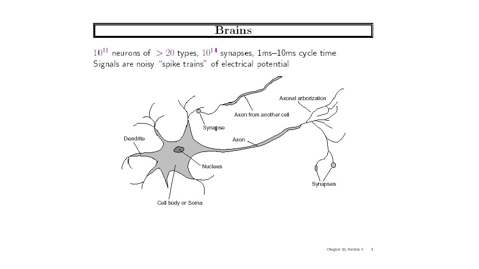
Neural Net Learning • Motivated by studies of the brain. • A network of “artificial neurons” that learns a function. • Doesn’t have clear decision rules like decision trees, but highly successful in many different applications. (e. g. face detection) • We use them frequently in our research. • I’ll be using algorithms from http: //www. cs. mtu. edu/~nilufer/classes/cs 4811/2016 -spring/lectureslides/cs 4811 -neural-net-algorithms. pdf 16

Common activation functions φ logistic linear REctified Linear Unit (RELU) tanh Leaky RELU

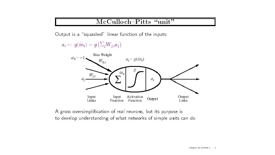
Simple Feed-Forward Perceptrons x 1 in = (∑ Wj xj) + out = g[in] W 1 g(in) x 2 out W 2 g is the activation function It can be a step function: g(x) = 1 if x >=0 and 0 (or -1) else. It can be a sigmoid function: g(x) = 1/(1+exp(-x)). The sigmoid function is differentiable and can be used in a gradient descent algorithm to update the weights. and other things…

Gradient Descent takes steps proportional to the negative of the gradient of a function to find its local minimum • Let X be the inputs, y the class, W the weights • in = ∑ Wj xj • Err = y – g(in) • E = ½ Err 2 is the squared error to minimize • E/ Wj = Err * Err/ Wj = Err * / Wj(g(in))(-1) • = -Err * g’(in) * xj • The update is Wj <- Wj + α * Err * g’(in) * xj • α is called the learning rate.

Simple Feed-Forward Perceptrons x 1 W 1 g(in) x 2 W 2 out repeat for each e in examples do in = (∑ Wj xj) + Err = y[e] – g[in] Wj = Wj + α Err g’(in) xj[e] until done Examples: A=[(. 5, 1. 5), +1], B=[(-. 5, . 5), -1], C=[(. 5, . 5), +1] Initialization: W 1 = 1, W 2 = 2, = -2 Note 1: when g is a step function, the g’(in) is removed. Note 2: later in back propagation, Err * g’(in) will be called We’ll let g(x) = 1 if x >=0 else -1

Graphically Examples: A=[(. 5, 1. 5), +1], B=[(-. 5, . 5), -1], C=[(. 5, . 5), +1] Initialization: W 1 = 1, W 2 = 2, = -2 W 2 Boundary is W 1 x 1 + W 2 x 2 + = 0 wrong boundary A B C W 1

Learning Examples: A=[(. 5, 1. 5), +1], B=[(-. 5, . 5), -1], C=[(. 5, . 5), +1] Initialization: W 1 = 1, W 2 = 2, = -2 A=[(. 5, 1. 5), +1] in =. 5(1) + (1. 5)(2) -2 = 1. 5 g(in) = 1; Err = 0; NO CHANGE B=[(-. 5, . 5), -1] In = (-. 5)(1) + (. 5)(2) -2 = -1. 5 g(in) = -1; Err = 0; NO CHANGE C=[(. 5, . 5), +1] in = (. 5)(1) + (. 5)(2) – 2 = -. 5 g(in) = -1; Err = 1 -(-1)=2 repeat for each e in examples do in = (∑ Wj xj) + Err = y[e] – g[in] Wj = Wj + α Err g’(in) xj[e] until done Let α=. 5 W 1 <- W 1 +. 5(2) (. 5) leaving out g’ <- 1 + 1(. 5) = 1. 5 W 2 <- W 2 +. 5(2) (. 5) <- 2 + 1(. 5) = 2. 5 <- +. 5(+1 – (-1)) <- -2 +. 5(2) = -1

Graphically Examples: A=[(. 5, 1. 5), +1], B=[(-. 5, . 5), -1], C=[(. 5, . 5), +1] Initialization: W 1 = 1, W 2 = 2, = -2 W 2 a wrong boundary Boundary is W 1 x 1 + W 2 x 2 + = 0 A B C W 1 approximately correct boundary

Back Propagation • Simple single layer networks with feed forward learning were not powerful enough. • Could only produce simple linear classifiers. • More powerful networks have multiple hidden layers. • The learning algorithm is called back propagation, because it computes the error at the end and propagates it back through the weights of the network to the beginning.

Let’s break it into steps.

Initialize layer 1 x 2 x 3 w 11 w 21 w 31 2 n 1 n 2 3=L w 1 f w 2 f nf

Forward Computation layer 1 x 2 x 3 w 11 w 21 w 31 2 n 1 n 2 g(inn 1) = an 1 3=L w 1 f nf w 2 f g(inn 2) = an 2 g(innf) = anf

Backward Propagation 1 • Node nf is the only node in our output layer. • Compute the error at that node and multiply by the derivative of the weighted input sum to get the change delta. layer 1 x 2 x 3 w 11 w 21 w 31 2 n 1 n 2 3=L w 1 f w 2 f nf

Backward Propagation 2 ht • At each of the other layers, the deltas use • the derivative of its input sum • the sum of its output weights • the delta computed for the output error layer 1 x 2 x 3 w 11 w 21 w 31 2 n 1 n 2 3=L w 1 f w 2 f nf If there were two output nodes, there would be a summation.

Backward Propagation 3 Now that all the deltas are defined, the weight updates just use them. layer 1 x 2 x 3 w 11 w 21 w 31 2 n 1 n 2 3=L w 1 f w 2 f nf ai i wij j

Back Propagation Summary • Compute delta values for the output units using observed errors. • Starting at the output-1 layer • repeat • propagate delta values back to previous layer • till done with all layers • update weights for all layers • This is done for all examples and multiple epochs, till convergence or enough iterations.

Time taken to build model: 16. 2 seconds Correctly Classified Instances 307 80. 3665 % (did not boost) Incorrectly Classified Instances 75 19. 6335 % Kappa statistic 0. 6056 Mean absolute error 0. 1982 Root mean squared error 0. 41 Relative absolute error 39. 7113 % Root relative squared error 81. 9006 % Total Number of Instances 382 TP Rate 0. 706 0. 897 W Avg. 0. 804 FP Rate 0. 103 0. 294 0. 2 === Confusion Matrix === a b <-- classified as 132 55 | a = cal 20 175 | b = dor Precision Recall F-Measure ROC Area Class 0. 868 0. 706 0. 779 0. 872 cal 0. 761 0. 897 0. 824 0. 872 dor 0. 814 0. 802 0. 872

Multi-Classification

Solution • Traditional Method: 1 -vs-other method • Too slow. If we have n-classes, we need to train n models • Performance is not great, because the sample size is different for positive and negative classes • Multiple Neurons • Use n output neuron to correspond n classes. • Easy, fast, and robust • Problem: how to model the probability? The values in the neural network can be negative or greater than 1.

Softmax: normalized exponential Input: vector of reals Output: probability distribution z softmax([1, 2, 7, 3, 2]): Calculate ex: [2. 72, 7. 39, 1096. 63, 20. 09, 7. 39] Calculate sum(ex): 2. 72+7. 39+1096. 63+20. 09+7. 39 = 1134. 22 Normalize: ex/sum(ex) = [0. 002, 0. 007, 0. 967, 0. 017, 0. 007] Result is a vector of reals.

A Simple Example Here, we will go over a simple 2 -layer neural network (no bias).

Mini-batch for Machine Learning • We use a matrix to represent data. • If there are 10, 000 images, and each image contains 784 features, we can use a 10, 000 x 784 matrix to represent the whole dataset. • Hard to load a large dataset at once; so, we can split the dataset into smaller batches. • For instance, in homework 5, we use batch size 128. Then, each batch contains 128 images, and the corresponding data is stored in a 128 x 784 matrix. • Then, we can feed batches one-by-one to the ML model, and train it for each batch.

Here, we use batch size of 4, and we only visualize the first sample for simplicity. Neural Network Easy Example 0. 7 1 First pixel 3 Second pixel 2 0. 1 -2. 3 -2. 1 0. 5 Third pixel 4 1 -0. 2 -0. 5 3 Input Layer 2 4 . . . 1 -st Layer (Re. LU) 1 0. 5 0. 1 1 -2. 3 -0. 5 Output Layer with Softmax 0. 7 -2. 1 0. 1 -0. 2

[Example] Forward Pass -6. 0 0 1 3 0. 15 0. 1 0. 7 . 61 0. 1 -2. 3 2 -2. 1 0. 5 4 3 Input Layer 2 4 . . . 1 1. 5 -0. 5 1. 5 . 39 -0. 2 Output Layer with Softmax 1 -st Layer (Re. LU) 1 0. 5 0. 1 1 -2. 3 -0. 5 -0. 3 0 1. 5 . . 0. 61 0. 39 0. 7 -2. 1 0. 1 -0. 2 . .

[Example] Ground Truth and Loss 0. 15 0 1 3 0. 1 0. 7 0. 1 -2. 3 Ground truth . 61 1 0. 39 2 -2. 1 0. 5 4 3. . . 0 . 39 1 -0. 2 1. 5 -0. 5 Input Layer 2 4 -0. 3 1 -st Layer (Re. LU) 1 0. 5 0. 1 1 -2. 3 -0. 5 0 1. 5 . . -0. 39 Output Layer with Softmax 0. 7 -2. 1 0. 1 -0. 2 Label 0. 61 0. 39. .

Assume g’(. ) = 1 [Example] Backpropagation 0 1 3 0. 15 0. 7 0. 1 -2. 3 0. 39 -0. 39 . . 0 0 0. 585 -0. 585 . 61 0. 39 2 -2. 1 0. 5 4 . 39 1 3. . . -0. 2 1. 5 -0. 5 Input Layer 2 4 -0. 3 1 -st Layer (Re. LU) 1 0. 5 0. 1 1 -2. 3 -0. 5 0 1. 5 . . -0. 39 Output Layer with Softmax 0. 7 -2. 1 0. 1 -0. 2 1. 092 0. 117 . . 0. 61 0. 39. .

0 0. 117 . . Backpropagation [Cont. ] 0 1 0 0. 351 0 0. 234 0 0. 468 3 0. 7 1. 092 (0) -2. 3 0. 1 -0. 39 . . 0 0 0. 585 -0. 585 . 61 0. 39 2 0. 0585 0. 117 -0. 0585 . . . -2. 1 0. 5 4 3. . . -0. 3. 39 1 -0. 2 1. 5 -0. 5 Input Layer 2 4 . 0. 15 0. 39 0. 117 1 -st Layer (Re. LU) 1 0. 5 0. 1 1 -2. 3 -0. 5 0 1. 5 . . -0. 39 Output Layer with Softmax 0. 7 -2. 1 0. 1 -0. 2 1. 092 0. 117 . . 0. 61 0. 39. .

[Example] Update with Learning Rate 0. 15 0 1 0 0. 351 0 0. 234 0 0. 468 3 0. 1 1. 092 (0) -2. 3 . 5351 0. 1 1. 0234 -2. 3 -0. 4532 4 -2. 1 0. 39 0 0 0. 585 -0. 585 3. . . -0. 3. 39 1 1. 5 -0. 5 Input Layer 2 4 . 0. 1 . 61 2 0. 5 1 0. 7 0. 117 1 -st Layer (Re. LU) 1 0. 5 0. 1 1 -2. 3 -0. 5 -0. 2 -0. 39 Output Layer with Softmax 0. 7 -2. 1 0. 1 -0. 2 0. 7 -2. 1 0. 1585 -0. 2585

[Example] Done 0. 7 1 3 0. 1585 -2. 3 2 -2. 1 . 5351 4 1. 0234 -0. 2585 -0. 4532 3 Input Layer 2 4 . . . 1 -st Layer (Re. LU) 1 0. 5351 0. 1 1. 0234 -2. 3 -0. 4532 Output Layer with Softmax 0. 7 -2. 1 0. 1585 -0. 2585

Think: What will happen if we go forward again? 0. 7 1 3 0. 1585 -2. 3 2 -2. 1 . 5351 4 1. 0234 -0. 2585 -0. 4532 3 Input Layer 2 4 . . . 1 -st Layer (Re. LU) 1 0. 5351 0. 1 1. 0234 -2. 3 -0. 4532 Output Layer with Softmax 0. 7 -2. 1 0. 1585 -0. 2585

Think: What will happen if we go forward again? 0. 292 0 1 3 0. 1 0. 7 The final output is closer to the actual label . . . -0. 475 -2. 1 1. 84 1 -st Layer (Re. LU) 1 0. 5351 0. 1 1. 0234 -2. 3 -0. 4532 Previous Output -0. 3 0 . 32 1. 0234 -0. 4532 3 . 61 0. 1585 -2. 3 . 5351 Input Layer 2 4 1 . 68 2 4 0. 15 -0. 2585 Output Layer with Softmax Label 0. 7 -2. 1 0. 1585 -0. 2585 . 39

Tricks for Neural Network

Problem: Under and Overfitting Underfitting: model not powerful enough, too much bias Overfitting: model too powerful, fits to noise, doesn’t generalize well Want the happy medium, how?

Weight decay: neural network regularization ● Subtract a little bit of weight every iteration

Momentum: speeding up SGD If we keep moving in same direction we should move further every round Before: Δwt = -∂/∂wt L(wt) Now: Δwt = -∂/∂wt L(wt) + mΔwt-1 wt+1 = wt + α Δwt Side effect: smooths out updates if gradient is in different directions

NN updates with weight decay and momentum Δw’t = -∂/∂wt L(wt) - λwt + mΔw’t-1 Gradient of loss Weight decay wt+1 = wt + α Δw’t Learning rate Momentum

Activations

Linear Activation ●

Logistic Activation ●

Re. LU Activation ●

Visualization with Re. LU https: //www. youtube. com/channel/UCYO_jab_esu. FRV 4 b 17 AJt. Aw

Leaky. Re. LU Activation ● ● No information loss (compared to Re. LU) Solves “dying Re. LU” problem (i. e. all neurons output 0) Similar to Re. LU, pays less attention to less important neurons Not always better than Re. LU

CSE 455 Homework 5 Neural Network Due: 05/28

MNIST: Handwriting recognition 50, 000 images of handwriting 28 x 1 (grayscale) Numbers 0 -9 10 class softmax regression Input is 784 pixel values Train the model > 95% accuracy

Functions You need to Code (classifier. c) void activate_matrix(matrix m, ACTIVATION a) void gradient_matrix(matrix m, ACTIVATION a, matrix d) matrix forward_layer(layer *l, matrix in) matrix backward_layer(layer *l, matrix delta) void update_layer(layer *l, double rate, double momentum, double decay) Run Experiments and Write a Report (hw 5. pdf) Play around with tryhw 5. py file, and answer the questions. Save your question to a PDF file and submit to Canvas for grading.

Important Data Structure (image. h) typedef enum{LINEAR, LOGISTIC, RELU, LRELU, SOFTMAX} ACTIVATION; typedef struct { matrix in; // Saved input to a layer matrix w; // Current weights for a layer matrix dw; // Current weight updates matrix v; // Past weight updates (for use with momentum) matrix out; // Saved output from the layer ACTIVATION activation; // Activation the layer uses } layer; typedef struct { layer *layers; int n; } model;

Useful Matrix manipulation functions (matrix. c) matrix_mult_matrix(matrix a, matrix b); matrix transpose_matrix(matrix m); matrix axpy_matrix(double a, matrix x, matrix y); // a * x + y

Forward Pass in Homework forward_model forward_layer Input: layer l, data in Input: model m, data X X = in * l->w forward_layer activation_matrix (X, l->activation) Output

Backward Pass in Homework backward_model backward_layer Input: layer l, matrix delta Input: model m, matrix d gradient_matrix backward_layer Output

Weight Update in Homework update_model update_layer Output update_layer

TODO void activate_matrix(matrix m, ACTIVATION a) for(i = 0; i < m. rows; ++i){ Apply activation “a” to the matrix “m” double sum = 0; for(j = 0; j < m. cols; ++j){ double x = m. data[i][j]; if(a == LOGISTIC){ // TODO m. data[i][j] should equals 1 / (1 + exp(-x)); } else if (a == RELU){ // TODO m. data[i][j] should equals x if x > 0; otherwise, it should equal 0 } else if (a == LRELU){ // TODO m. data[i][j] should equals x if x > 0; otherwise, it should equal 0. 1 * x. } else if (a == SOFTMAX){ // TODO m. data[i][j] should equals exp(x) here, and we will normalize it later. } sum += m. data[i][j]; } if (a == SOFTMAX) { // TODO: have to normalize by sum if we are using SOFTMAX // for all the possible j, we should normalize it as m. data[i][j] /= sum; } }

TODO void gradient_matrix(matrix m, ACTIVATION a, matrix d) int i, j; for(i = 0; i < m. rows; ++i){ for(j = 0; j < m. cols; ++j){ double x = m. data[i][j]; // TODO: multiply the correct element of d by the gradient // if a is SOFTMAX or a is LINEAR, we should do nothing (multiply by 1) // if a is LOGISTIC, d. data[i][j] should times x * (1. 0 - x); // if a is RELU and x <= 0, d. data[i][j] should be zero // if a is LRELU and x <= 0, d. data[i][j] should multiple 0. 1 } }

TODO matrix forward_layer(layer *l, matrix in) Given the input data “in” and layer “l”, calculate the output data. l->in = in; // Save the input for backpropagation // TODO: multiply input by weights and apply activation function. // Calculate out = in * l->w (note: matrix multiplication here) // Then, apply activate_matrix function to out with l->activation free_matrix(l->out); // free the old output l->out = out; return out; // Save the current output for gradient calculation

TODO matrix backward_layer(layer *l, matrix delta) // delta is Δout // TODO: modify it in place to be “g'(out) * delta” out with // gradient_matrix function. // You can use gradient_matrix function with “l->out” and “l->activation” to “delta” // TODO: then calculate d. L/dw and save it in l->dw free_matrix(l->dw); // Calculate xt as the transpose matrix of “l->in” // Calculate dw as xt times delta (matrix multiplication) // free matrix xt to avoid memory leak l->dw = dw; // TODO: finally, calculate d. L/dx and return it. (Similar to 1. 4. 2. Care memory leak) // Calculate dx = delta * (l->w)^T, return dx; where * is matrix multiplication and ^T is matrix transpose

TODO void update_layer(layer *l, double rate, double momentum, double decay) Given a layer “l”, learning rate, momentum, and decay rate, Update the weight (i. e. l->w) // Calculate Δw_t = d. L/dw_t - λw_t + mΔw_{t-1} // save it to l->v // Note that You can use axpy_matrix to perform the matrix summation/subtraction // Update l->w // l->w = rate * l->v + l->w Note the multiplication and summation in this slides all mean matrix multiplication or matrix summation.

Functions You Need to Know before Experiments For simplicity, we already filled the following functions for you. You should read and understand these functions (classifier. c) before running experiments. layer make_layer(int input, int output, ACTIVATION activation) matrix forward_model(model m, matrix X) void backward_model(model m, matrix d. L) void update_model(model m, double rate, double momentum, double decay) double accuracy_model(model m, data d) double cross_entropy_loss(matrix y, matrix p) void train_model(model m, data d, int batch, int iters, double rate, double momentum, double decay)

Get the Data 1. Download, Unzip, and Prepare the MNIST Dataset wget https: //pjreddie. com/media/files/mnist_train. tar. gz wget https: //pjreddie. com/media/files/mnist_test. tar. gz tar xzf mnist_train. tar. gz tar xzf mnist_test. tar. gz find train -name *. png > mnist. train find test -name *. png > mnist. test 2. Download, Unzip, and Prepare the CIFAR-10 Dataset wget http: //pjreddie. com/media/files/cifar. tgz tar xzf cifar. tgz find cifar/train -name *. png > cifar. train find cifar/test -name *. png > cifar. test

Experiments (Write Your Answers to hw 5. pdf) 1. 2. Coding and Data prepare MNIST Experiments 1. Linear Softmax Model (1 -layer) 1. 2. 3. 2. Neural Network (2 -layer NNs and 3 -layer NNs) 1. 2. 3. 4. 3. Run the basic model Tune the learning rate Tune the decay Find the best activation Tune the learning rate Tune the decay for 3 -layer Neural Network Experiments for CIFAR-10 1. Neural Network (3 -layer NNs) 1. Tune the learning rate and decay