Image Stitching II Linda Shapiro CSE 455 RANSAC

Image Stitching II Linda Shapiro CSE 455

RANSAC for Homography Initial Matched Points

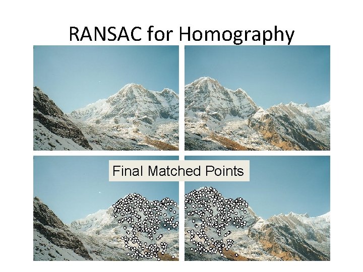
RANSAC for Homography Final Matched Points

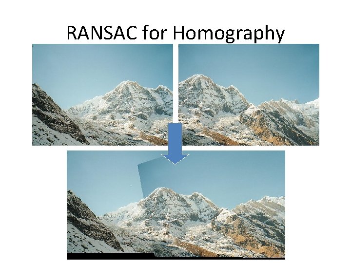
RANSAC for Homography

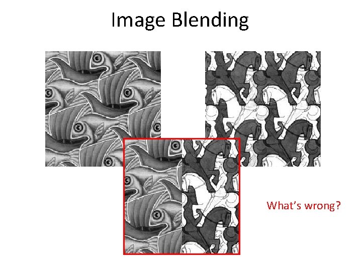
Image Blending What’s wrong?

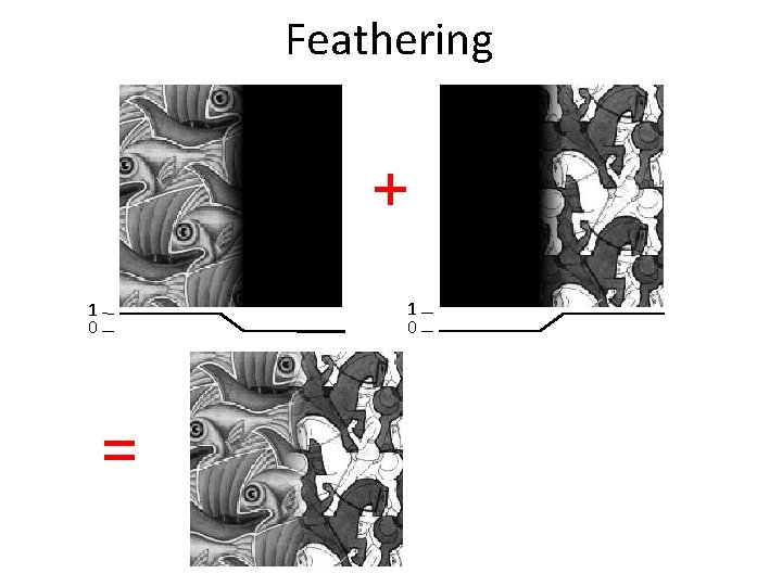
Feathering + 1 0 =

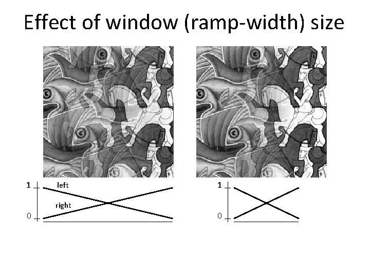
Effect of window (ramp-width) size 1 0 left right 1 0

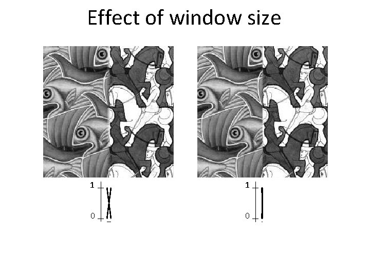
Effect of window size 1 1 0 0

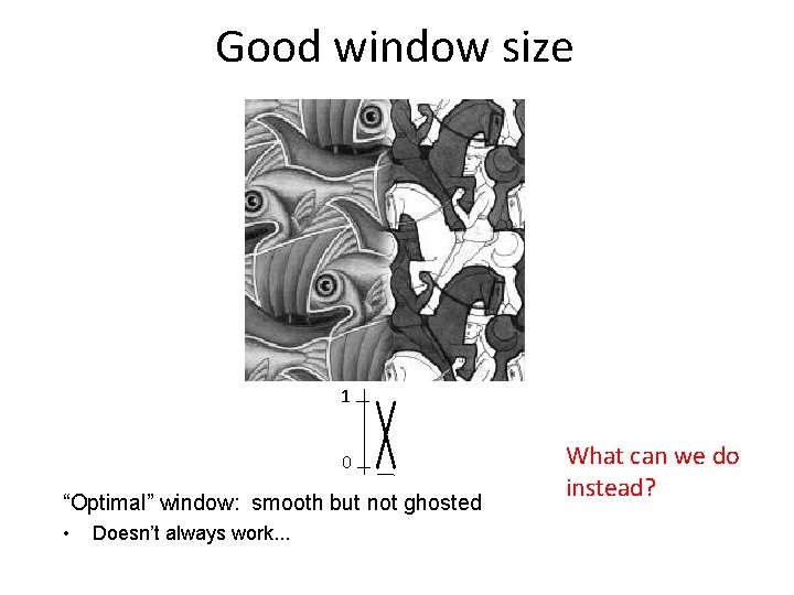
Good window size 1 0 “Optimal” window: smooth but not ghosted • Doesn’t always work. . . What can we do instead?

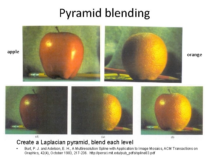
Pyramid blending apple orange Create a Laplacian pyramid, blend each level • Burt, P. J. and Adelson, E. H. , A Multiresolution Spline with Application to Image Mosaics, ACM Transactions on Graphics, 42(4), October 1983, 217 -236. http: //persci. mit. edu/pub_pdfs/spline 83. pdf

Forming a Gaussian Pyramid • Start with the original image G 0 • Perform a local Gaussian weighted averaging function in a neighborhood about each pixel, sampling so that the result is a reduced image of half the size in each dimension. • Do this all the way up the pyramid Gl = REDUCE(Gl-1) • Each level l node will represent a weighted average of a subarray of level l.

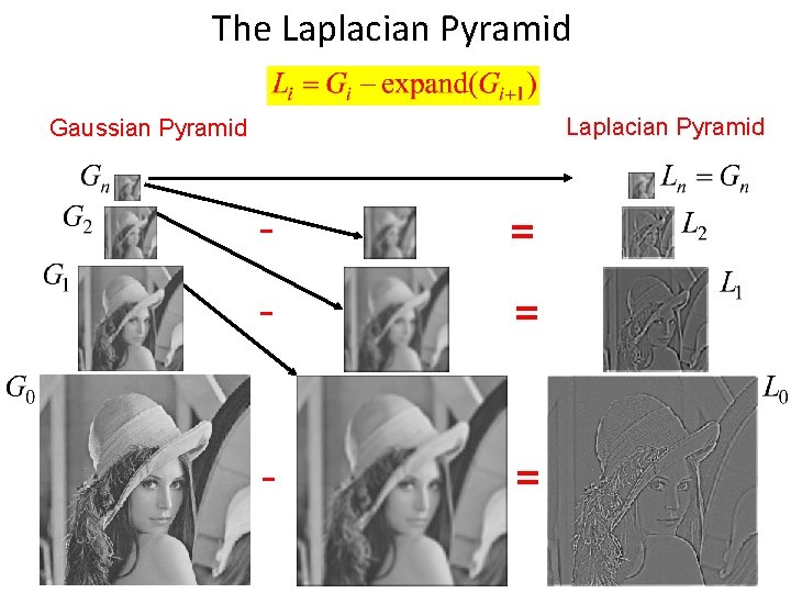
Making the Laplacians • We want to subtract each level of the pyramid from the next lower one. • But they are different sizes! • In order to do the subtraction, we perform an interpolation process. • We interpolate new samples between those of a given image to make it big enough to subtract. • The operation is called EXPAND.

The Laplacian Pyramid Gaussian Pyramid - = - =

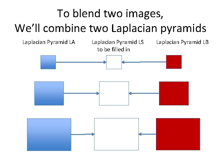
To blend two images, We’ll combine two Laplacian pyramids Laplacian Pyramid LA Laplacian Pyramid LS to be filled in Laplacian Pyramid LB

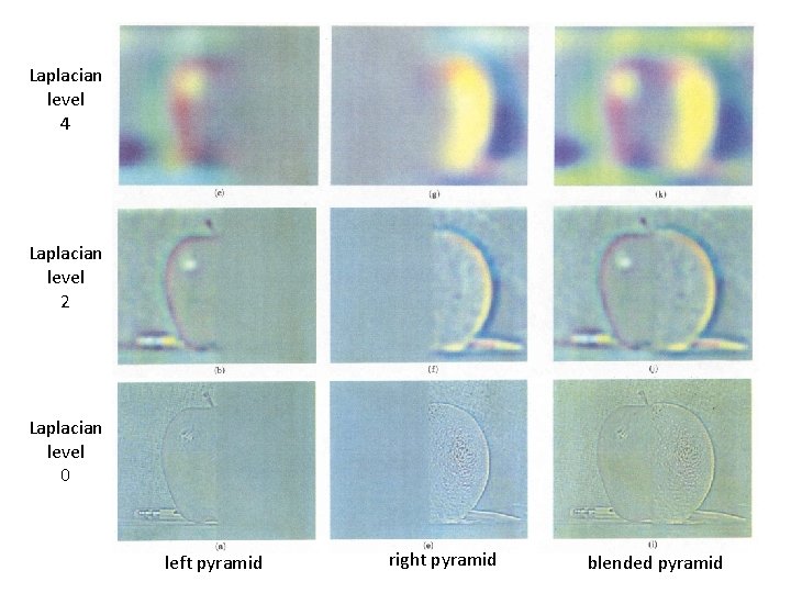
Forming the New Pyramid • Laplacian pyramids LB and LB are constructed for images A and B, respectively. • A third Laplacian pyramid LS is constructed by copying nodes from the left half of LA to the corresponding nodes of LS and nodes from the right half of LB to the right half of LS. • Nodes along the center line are set equal to the average of corresponding LA and LB nodes

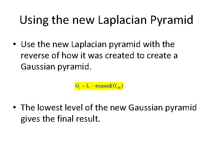
Using the new Laplacian Pyramid • Use the new Laplacian pyramid with the reverse of how it was created to create a Gaussian pyramid. • The lowest level of the new Gaussian pyramid gives the final result.

Laplacian level 4 Laplacian level 2 Laplacian level 0 left pyramid right pyramid blended pyramid

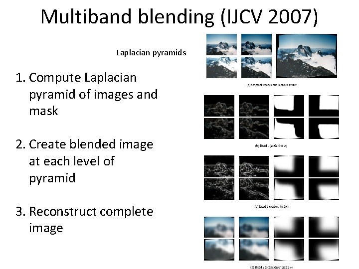
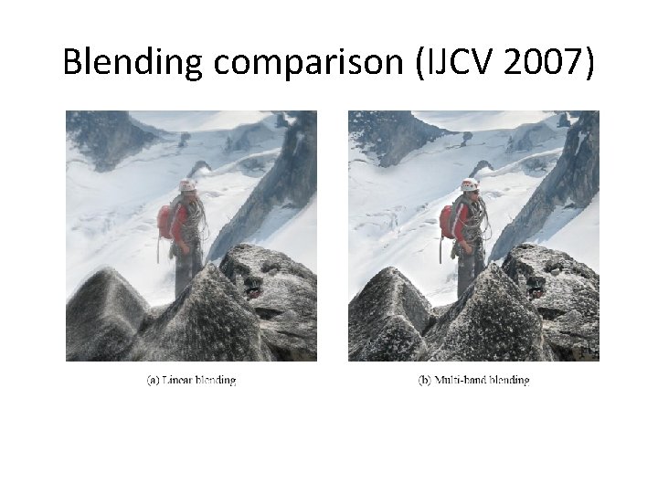
Multiband blending (IJCV 2007) Laplacian pyramids 1. Compute Laplacian pyramid of images and mask 2. Create blended image at each level of pyramid 3. Reconstruct complete image

Blending comparison (IJCV 2007)

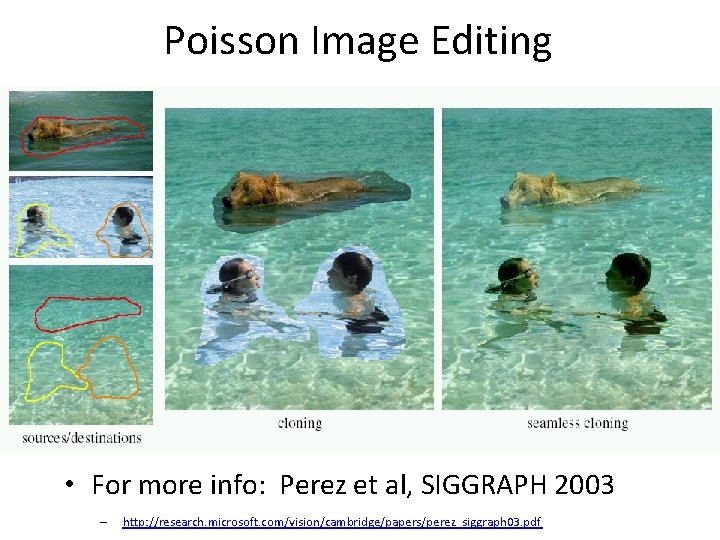
Poisson Image Editing • For more info: Perez et al, SIGGRAPH 2003 – http: //research. microsoft. com/vision/cambridge/papers/perez_siggraph 03. pdf

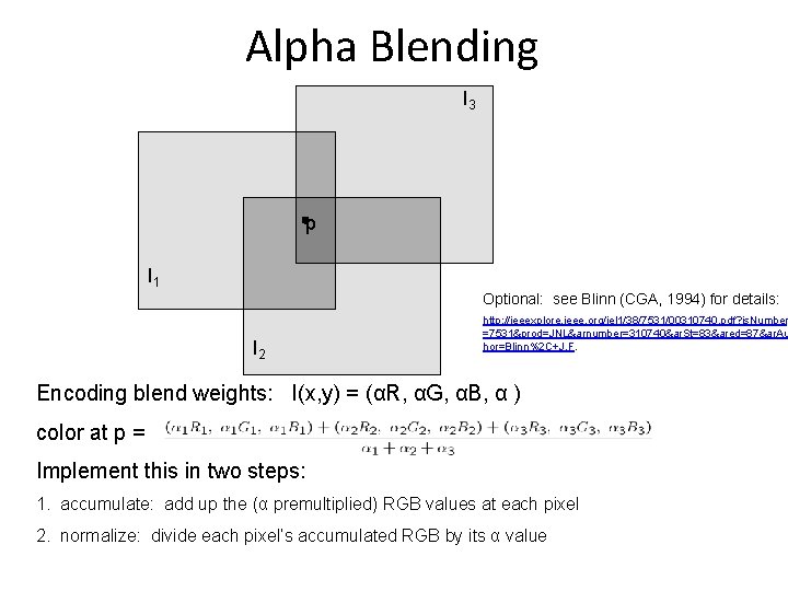
Alpha Blending I 3 p I 1 Optional: see Blinn (CGA, 1994) for details: I 2 http: //ieeexplore. ieee. org/iel 1/38/7531/00310740. pdf? is. Number =7531&prod=JNL&arnumber=310740&ar. St=83&ared=87&ar. Au hor=Blinn%2 C+J. F. Encoding blend weights: I(x, y) = (αR, αG, αB, α ) color at p = Implement this in two steps: 1. accumulate: add up the (α premultiplied) RGB values at each pixel 2. normalize: divide each pixel’s accumulated RGB by its α value

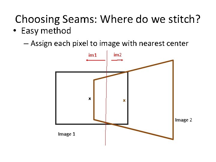
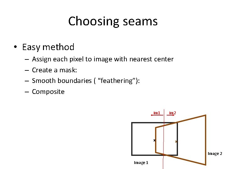
Choosing Seams: Where do we stitch? • Easy method – Assign each pixel to image with nearest center im 1 x im 2 x Image 2 Image 1

Choosing seams • Easy method – – Assign each pixel to image with nearest center Create a mask: Smooth boundaries ( “feathering”): Composite im 1 x im 2 x Image 2 Image 1

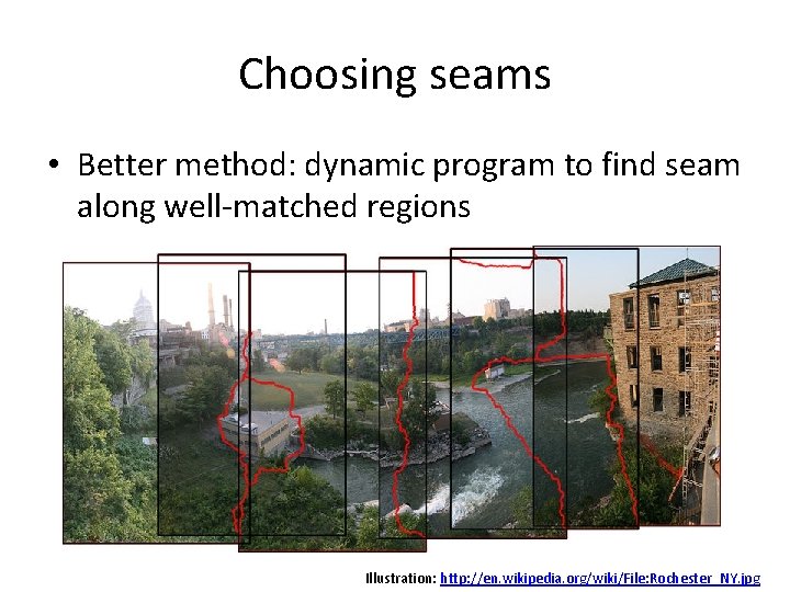
Choosing seams • Better method: dynamic program to find seam along well-matched regions Illustration: http: //en. wikipedia. org/wiki/File: Rochester_NY. jpg

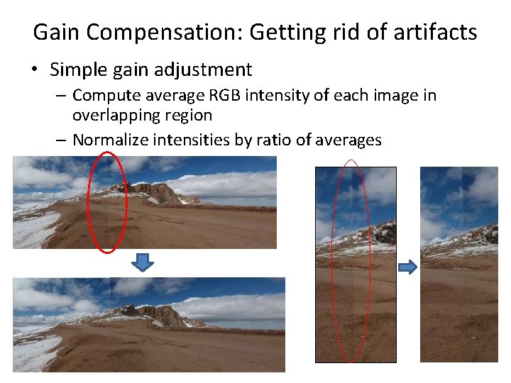
Gain Compensation: Getting rid of artifacts • Simple gain adjustment – Compute average RGB intensity of each image in overlapping region – Normalize intensities by ratio of averages

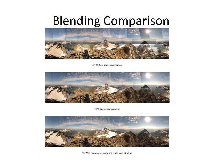
Blending Comparison

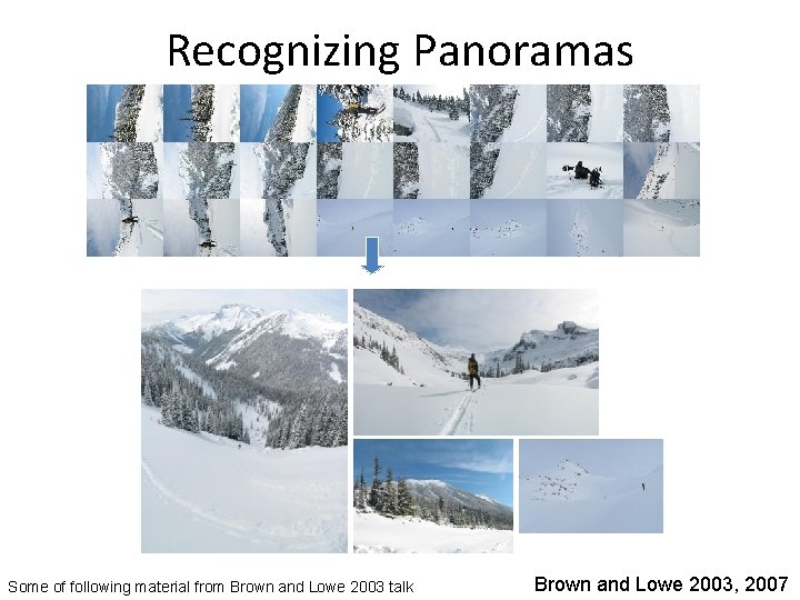
Recognizing Panoramas Some of following material from Brown and Lowe 2003 talk Brown and Lowe 2003, 2007

Recognizing Panoramas Input: N images 1. Extract SIFT points, descriptors from all images 2. Find K-nearest neighbors for each point (K=4) 3. For each image a) Select M candidate matching images by counting matched keypoints (m=6) b) Solve homography Hij for each matched image

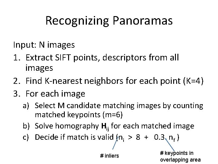
Recognizing Panoramas Input: N images 1. Extract SIFT points, descriptors from all images 2. Find K-nearest neighbors for each point (K=4) 3. For each image a) Select M candidate matching images by counting matched keypoints (m=6) b) Solve homography Hij for each matched image c) Decide if match is valid (ni > 8 + 0. 3 nf ) # inliers # keypoints in overlapping area

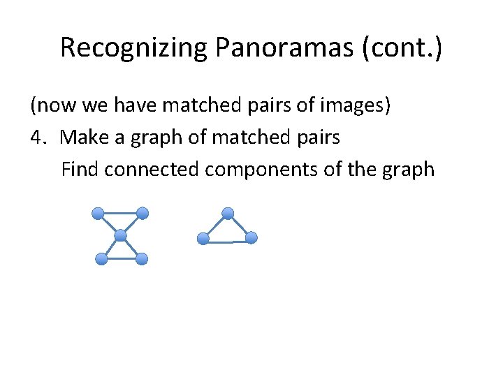
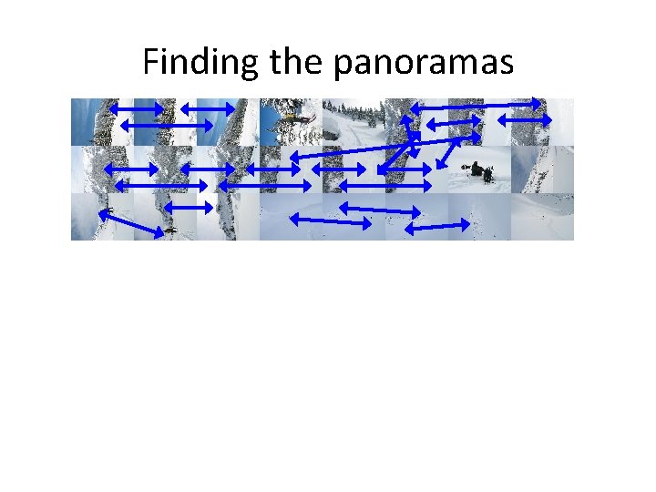
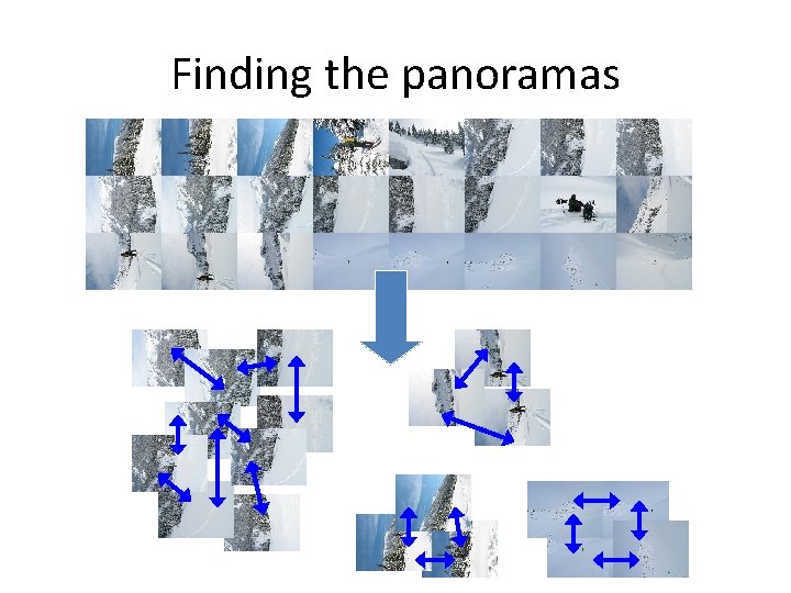
Recognizing Panoramas (cont. ) (now we have matched pairs of images) 4. Make a graph of matched pairs Find connected components of the graph

Finding the panoramas

Finding the panoramas

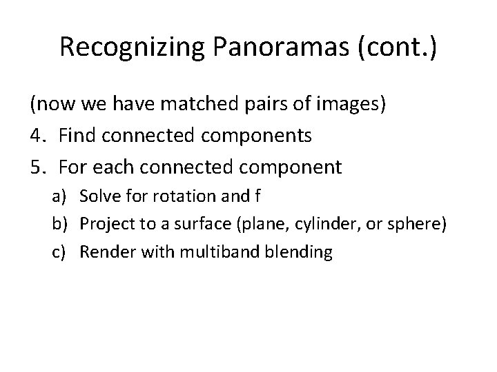
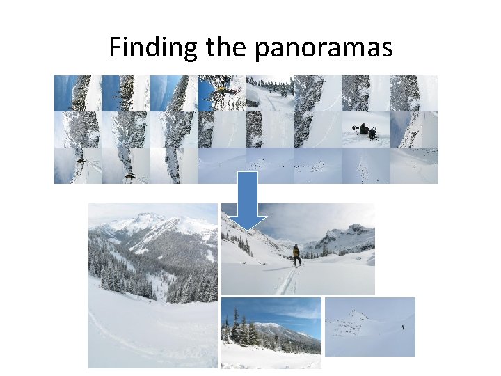
Recognizing Panoramas (cont. ) (now we have matched pairs of images) 4. Find connected components 5. For each connected component a) Solve for rotation and f b) Project to a surface (plane, cylinder, or sphere) c) Render with multiband blending

Finding the panoramas