Learning I Linda Shapiro CSE 455 1 Learning

Learning I Linda Shapiro CSE 455 1

Learning • AI/Vision systems are complex and may have many parameters. • It is impractical and often impossible to encode all the knowledge a system needs. • Different types of data may require very different parameters. • Instead of trying to hard code all the knowledge, it makes sense to learn it. 2

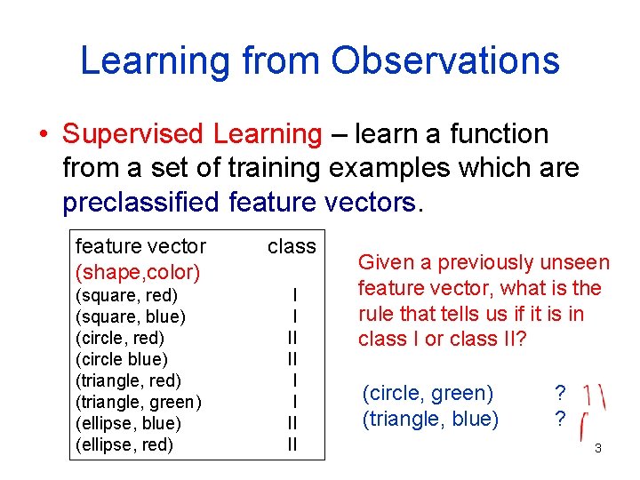
Learning from Observations • Supervised Learning – learn a function from a set of training examples which are preclassified feature vectors. feature vector (shape, color) class (square, red) (square, blue) (circle, red) (circle blue) (triangle, red) (triangle, green) (ellipse, blue) (ellipse, red) I I II II Given a previously unseen feature vector, what is the rule that tells us if it is in class I or class II? (circle, green) (triangle, blue) ? ? 3

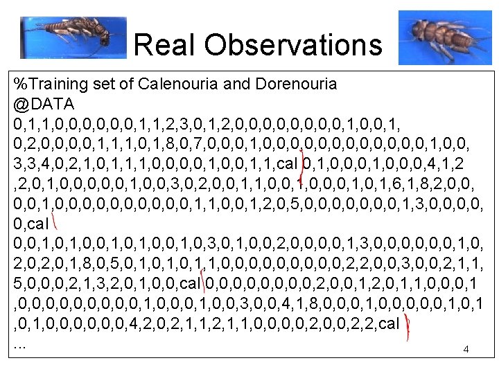
Real Observations %Training set of Calenouria and Dorenouria @DATA 0, 1, 1, 0, 0, 0, 1, 1, 2, 3, 0, 1, 2, 0, 0, 1, 0, 0, 1, 0, 2, 0, 0, 1, 1, 1, 0, 1, 8, 0, 7, 0, 0, 0, 1, 0, 0, 0, 1, 0, 0, 3, 3, 4, 0, 2, 1, 0, 1, 1, 1, 0, 0, 1, 1, cal 0, 1, 0, 0, 0, 4, 1, 2 , 2, 0, 1, 0, 0, 3, 0, 2, 0, 0, 1, 1, 0, 0, 0, 1, 6, 1, 8, 2, 0, 0, 1, 0, 0, 0, 1, 1, 0, 0, 1, 2, 0, 5, 0, 0, 1, 3, 0, 0, 0, cal 0, 0, 1, 0, 0, 1, 0, 3, 0, 1, 0, 0, 2, 0, 0, 1, 3, 0, 0, 0, 1, 0, 2, 0, 1, 8, 0, 5, 0, 1, 1, 0, 0, 0, 2, 2, 0, 0, 3, 0, 0, 2, 1, 1, 5, 0, 0, 0, 2, 1, 3, 2, 0, 1, 0, 0, cal 0, 0, 2, 0, 0, 1, 2, 0, 1, 1, 0, 0, 0, 1 , 0, 0, 0, 1, 0, 0, 3, 0, 0, 4, 1, 8, 0, 0, 0, 1, 0, 0, 0, 1, 0, 0, 0, 4, 2, 0, 2, 1, 1, 0, 0, 2, 2, cal. . . 4

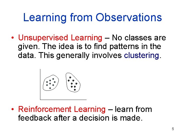
Learning from Observations • Unsupervised Learning – No classes are given. The idea is to find patterns in the data. This generally involves clustering. • Reinforcement Learning – learn from feedback after a decision is made. 5

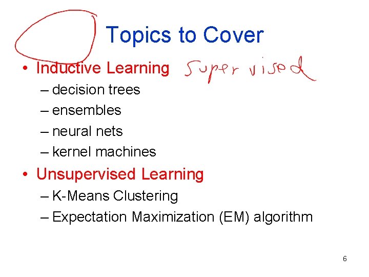
Topics to Cover • Inductive Learning – decision trees – ensembles – neural nets – kernel machines • Unsupervised Learning – K-Means Clustering – Expectation Maximization (EM) algorithm 6

Decision Trees • Theory is well-understood. • Often used in pattern recognition problems. • Has the nice property that you can easily understand the decision rule it has learned. 7

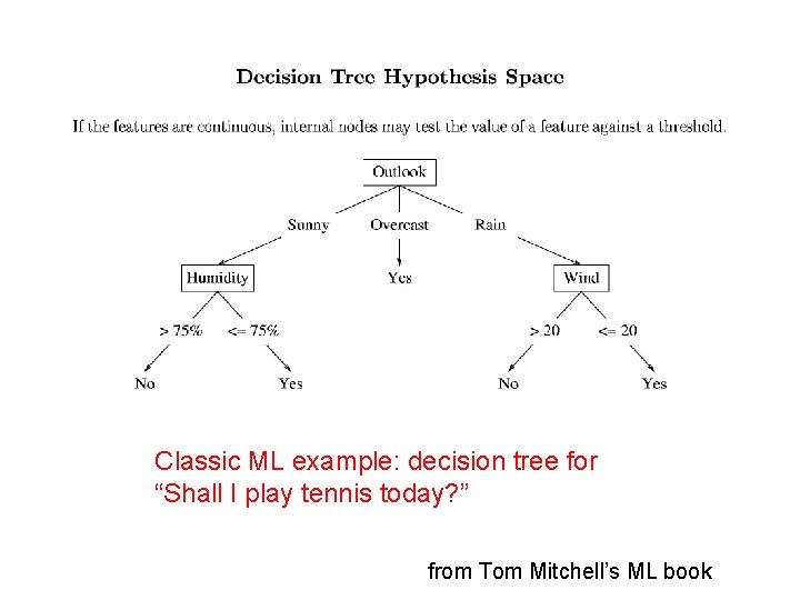
Classic ML example: decision tree for “Shall I play tennis today? ” from Tom Mitchell’s ML book 8

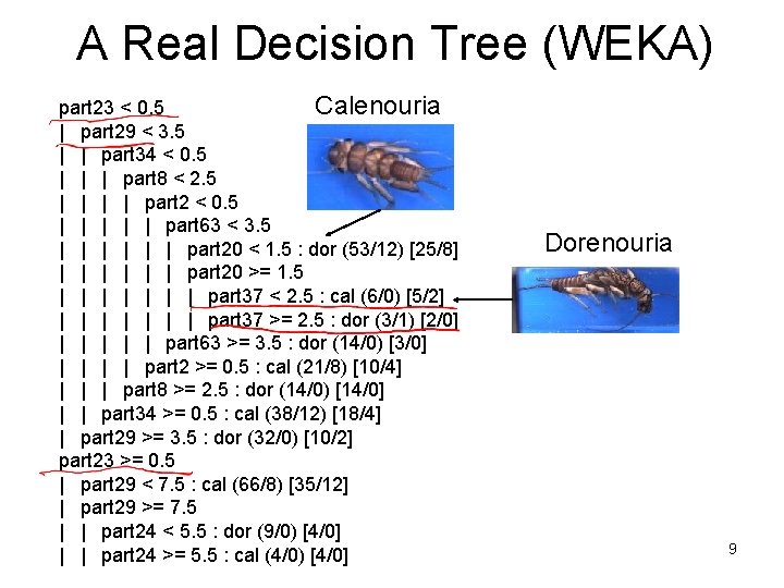
A Real Decision Tree (WEKA) Calenouria part 23 < 0. 5 | part 29 < 3. 5 | | part 34 < 0. 5 | | | part 8 < 2. 5 | | part 2 < 0. 5 | | | part 63 < 3. 5 | | | part 20 < 1. 5 : dor (53/12) [25/8] | | | part 20 >= 1. 5 | | | | part 37 < 2. 5 : cal (6/0) [5/2] | | | | part 37 >= 2. 5 : dor (3/1) [2/0] | | | part 63 >= 3. 5 : dor (14/0) [3/0] | | part 2 >= 0. 5 : cal (21/8) [10/4] | | | part 8 >= 2. 5 : dor (14/0) [14/0] | | part 34 >= 0. 5 : cal (38/12) [18/4] | part 29 >= 3. 5 : dor (32/0) [10/2] part 23 >= 0. 5 | part 29 < 7. 5 : cal (66/8) [35/12] | part 29 >= 7. 5 | | part 24 < 5. 5 : dor (9/0) [4/0] | | part 24 >= 5. 5 : cal (4/0) [4/0] Dorenouria 9

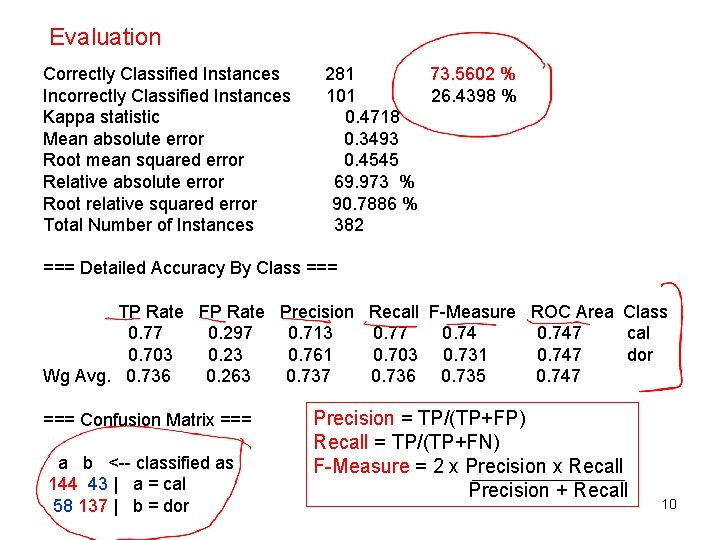
Evaluation Correctly Classified Instances Incorrectly Classified Instances Kappa statistic Mean absolute error Root mean squared error Relative absolute error Root relative squared error Total Number of Instances 281 73. 5602 % 101 26. 4398 % 0. 4718 0. 3493 0. 4545 69. 973 % 90. 7886 % 382 === Detailed Accuracy By Class === TP Rate FP Rate Precision Recall F-Measure ROC Area Class 0. 77 0. 297 0. 713 0. 77 0. 747 cal 0. 703 0. 23 0. 761 0. 703 0. 731 0. 747 dor Wg Avg. 0. 736 0. 263 0. 737 0. 736 0. 735 0. 747 === Confusion Matrix === a b <-- classified as 144 43 | a = cal 58 137 | b = dor Precision = TP/(TP+FP) Recall = TP/(TP+FN) F-Measure = 2 x Precision x Recall Precision + Recall 10

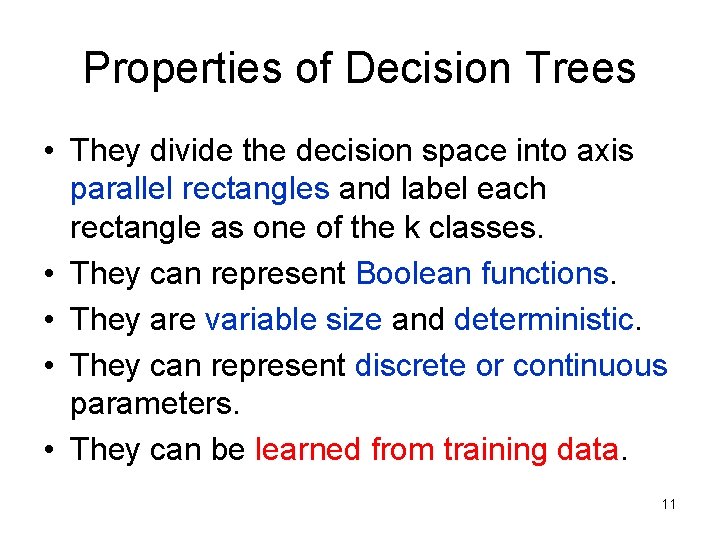
Properties of Decision Trees • They divide the decision space into axis parallel rectangles and label each rectangle as one of the k classes. • They can represent Boolean functions. • They are variable size and deterministic. • They can represent discrete or continuous parameters. • They can be learned from training data. 11

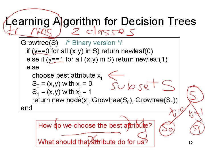
Learning Algorithm for Decision Trees Growtree(S) /* Binary version */ if (y==0 for all (x, y) in S) return newleaf(0) else if (y==1 for all (x, y) in S) return newleaf(1) else choose best attribute xj S 0 = (x, y) with xj = 0 S 1 = (x, y) with xj = 1 return new node(xj, Growtree(S 0), Growtree(S 1)) end How do we choose the best attribute? What should that attribute do for us? 12

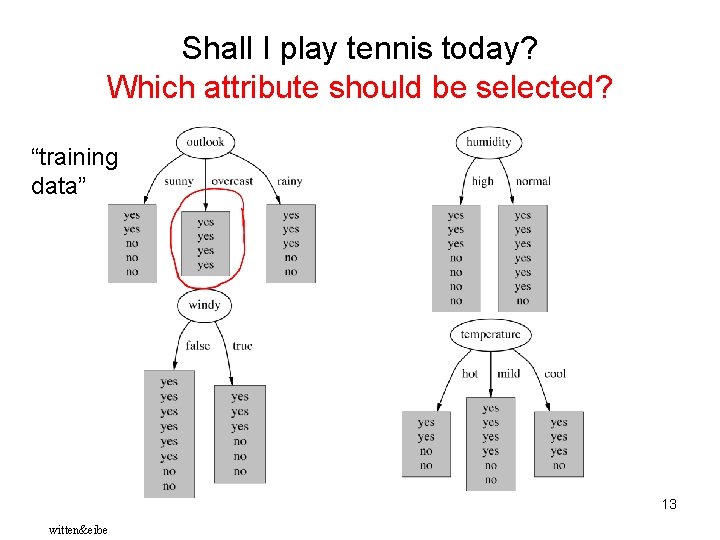
Shall I play tennis today? Which attribute should be selected? “training data” 13 witten&eibe

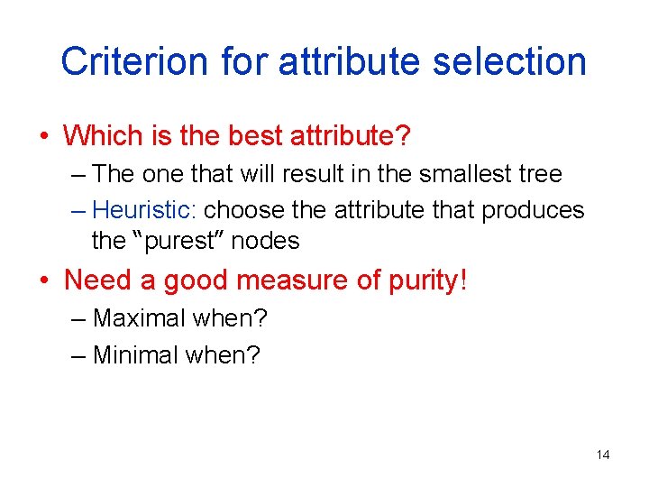
Criterion for attribute selection • Which is the best attribute? – The one that will result in the smallest tree – Heuristic: choose the attribute that produces the “purest” nodes • Need a good measure of purity! – Maximal when? – Minimal when? 14

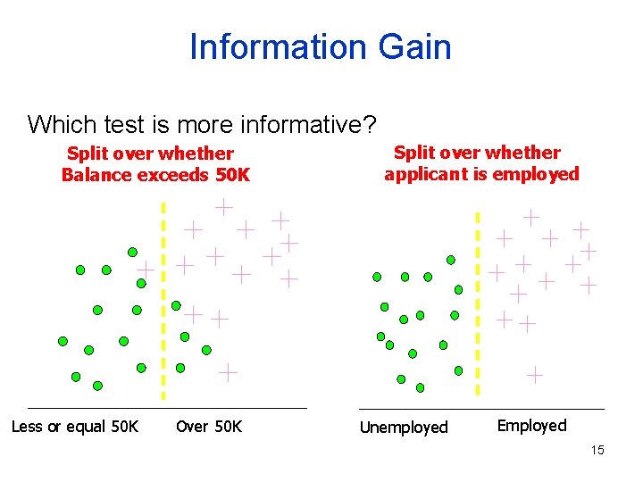
Information Gain Which test is more informative? Split over whether Balance exceeds 50 K Less or equal 50 K Over 50 K Split over whether applicant is employed Unemployed Employed 15

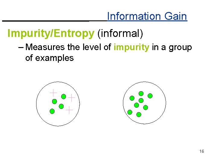
Information Gain Impurity/Entropy (informal) – Measures the level of impurity in a group of examples 16

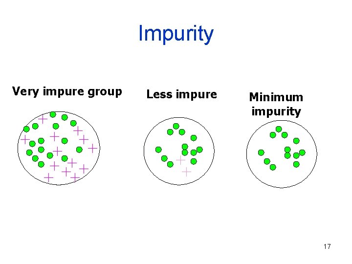
Impurity Very impure group Less impure Minimum impurity 17

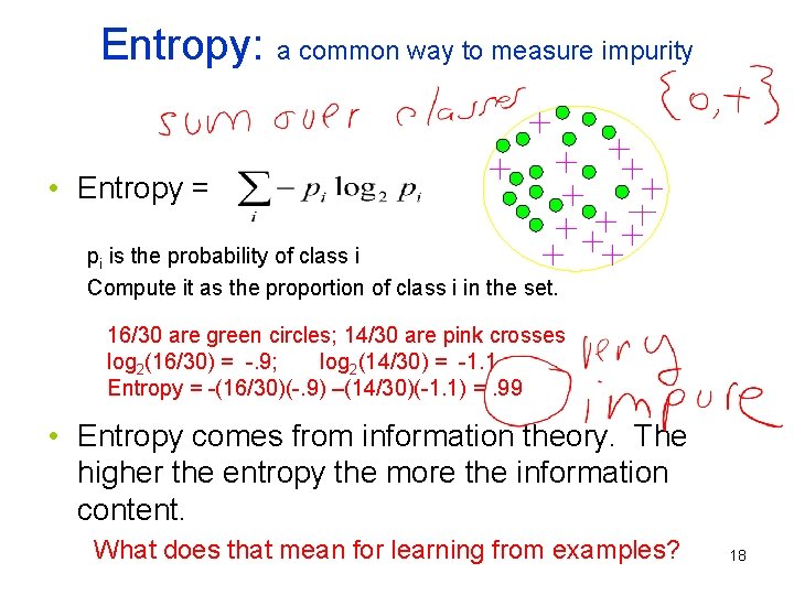
Entropy: a common way to measure impurity • Entropy = pi is the probability of class i Compute it as the proportion of class i in the set. 16/30 are green circles; 14/30 are pink crosses log 2(16/30) = -. 9; log 2(14/30) = -1. 1 Entropy = -(16/30)(-. 9) –(14/30)(-1. 1) =. 99 • Entropy comes from information theory. The higher the entropy the more the information content. What does that mean for learning from examples? 18

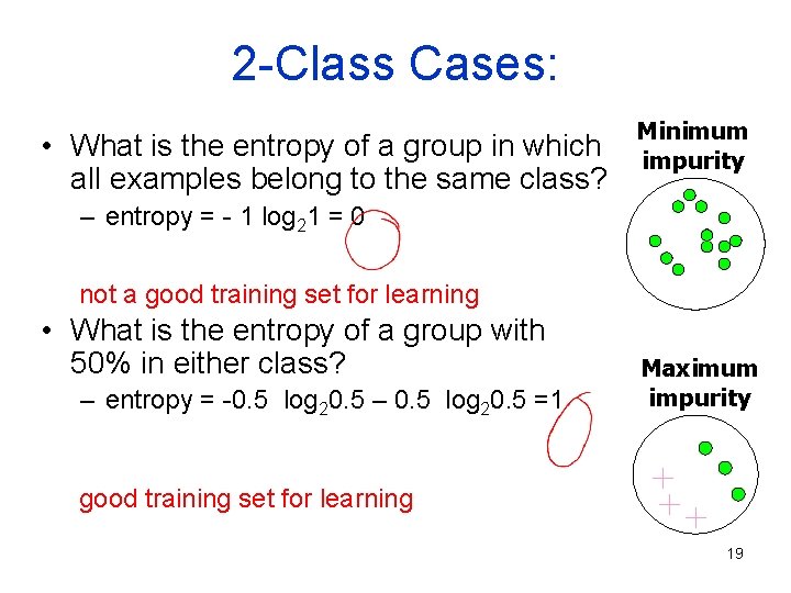
2 -Class Cases: • What is the entropy of a group in which all examples belong to the same class? Minimum impurity – entropy = - 1 log 21 = 0 not a good training set for learning • What is the entropy of a group with 50% in either class? – entropy = -0. 5 log 20. 5 – 0. 5 log 20. 5 =1 Maximum impurity good training set for learning 19

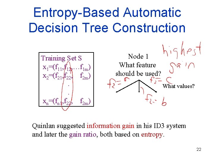
Information Gain • We want to determine which attribute in a given set of training feature vectors is most useful for discriminating between the classes to be learned. • Information gain tells us how important a given attribute of the feature vectors is. • We will use it to decide the ordering of attributes in the nodes of a decision tree. 20

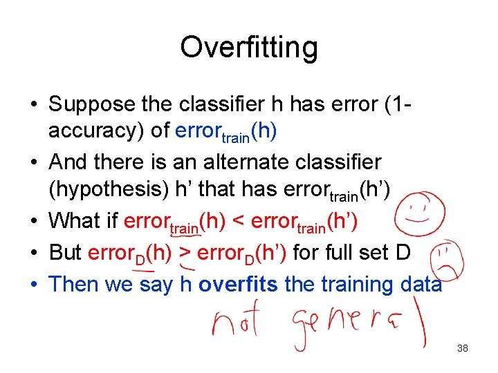
Calculating Information Gain = entropy(parent) – [average entropy(children)] parent entropy child entropy Entire population (30 instances) 17 instances child entropy (Weighted) Average Entropy of Children = Information Gain= 0. 996 - 0. 615 = 0. 38 13 instances for this split 21

Entropy-Based Automatic Decision Tree Construction Training Set S x 1=(f 11, f 12, …f 1 m) x 2=(f 21, f 22, f 2 m). . xn=(fn 1, f 22, f 2 m) Node 1 What feature should be used? What values? Quinlan suggested information gain in his ID 3 system and later the gain ratio, both based on entropy. 22

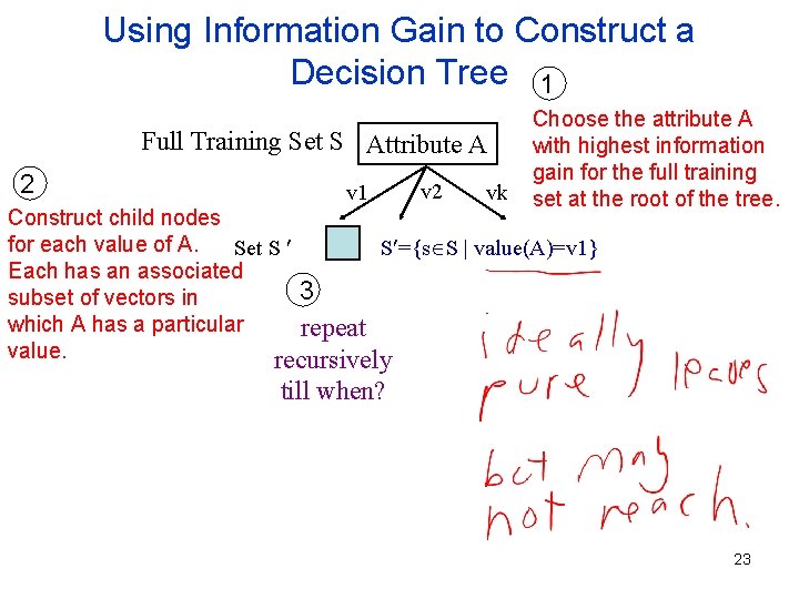
Using Information Gain to Construct a Decision Tree 1 Full Training Set S Attribute A 2 v 1 v 2 vk Choose the attribute A with highest information gain for the full training set at the root of the tree. Construct child nodes for each value of A. Set S S ={s S | value(A)=v 1} Each has an associated 3 subset of vectors in which A has a particular repeat value. recursively till when? 23

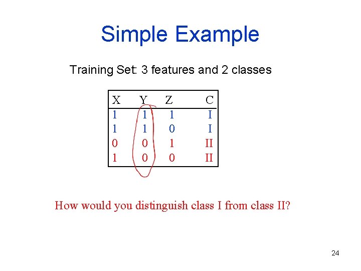
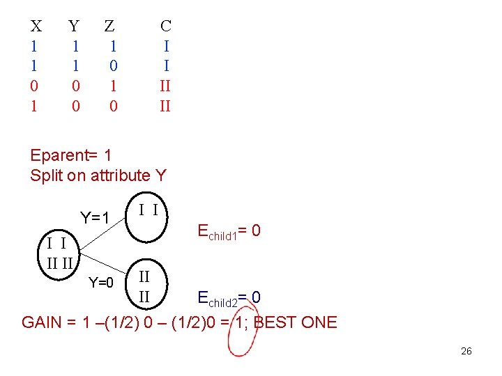
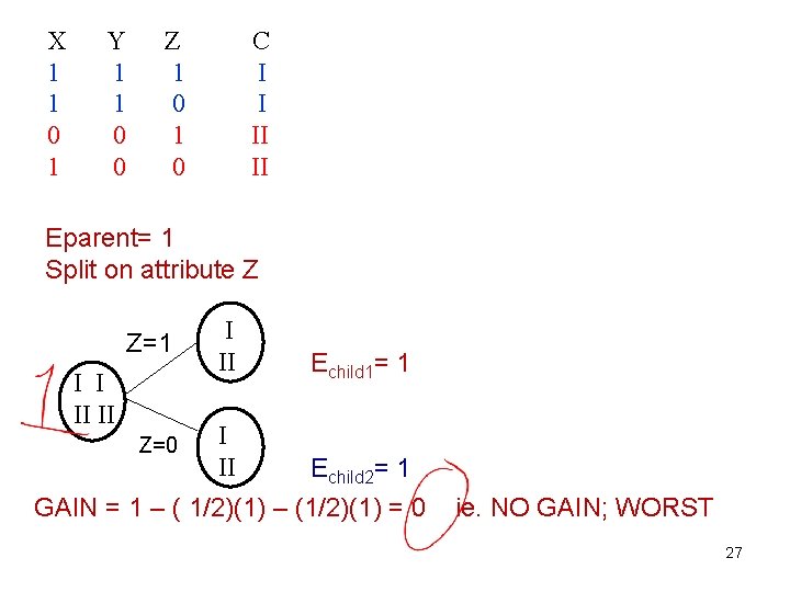
Simple Example Training Set: 3 features and 2 classes X 1 1 0 1 Y 1 1 0 0 Z 1 0 C I I II II How would you distinguish class I from class II? 24

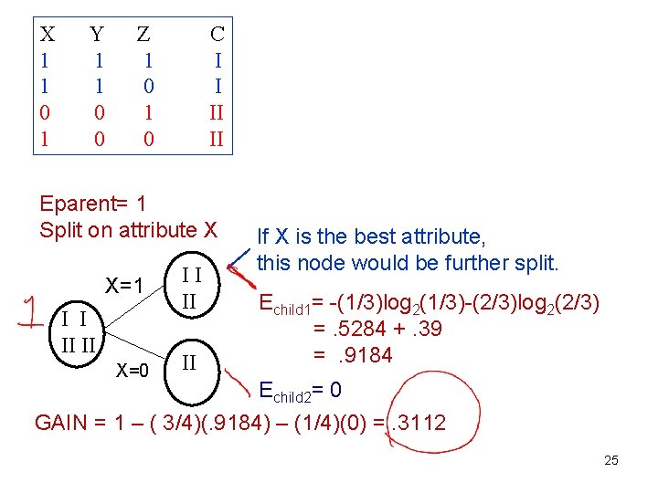
X 1 1 0 1 Y 1 1 0 0 Z 1 0 C I I II II Eparent= 1 Split on attribute X X=1 II II X=0 II I I II II If X is the best attribute, this node would be further split. Echild 1= -(1/3)log 2(1/3)-(2/3)log 2(2/3) =. 5284 +. 39 =. 9184 Echild 2= 0 GAIN = 1 – ( 3/4)(. 9184) – (1/4)(0) =. 3112 25

X 1 1 0 1 Y 1 1 0 0 Z 1 0 C I I II II Eparent= 1 Split on attribute Y Y=1 I I II II Y=0 I I Echild 1= 0 II II Echild 2= 0 GAIN = 1 –(1/2) 0 – (1/2)0 = 1; BEST ONE 26

X 1 1 0 1 Y 1 1 0 0 Z 1 0 C I I II II Eparent= 1 Split on attribute Z Z=1 I II Z=0 I II II Echild 1= 1 Echild 2= 1 GAIN = 1 – ( 1/2)(1) – (1/2)(1) = 0 ie. NO GAIN; WORST 27

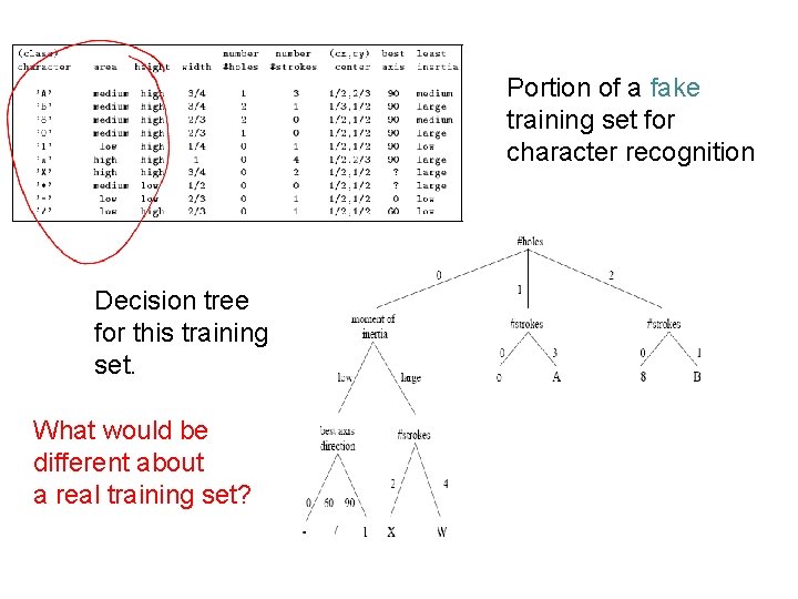
Portion of a fake training set for character recognition Decision tree for this training set. What would be different about a real training set?

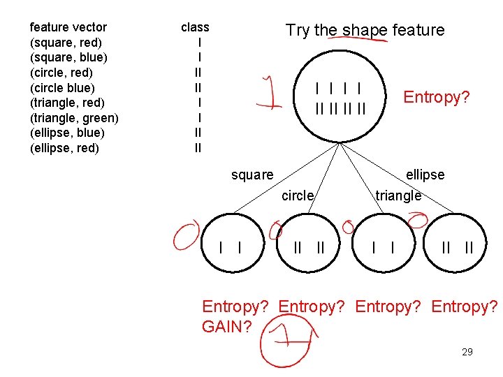
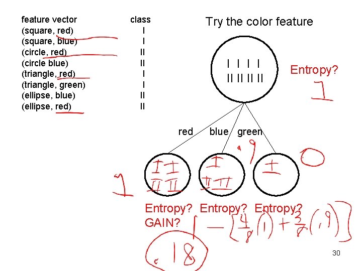
feature vector (square, red) (square, blue) (circle, red) (circle blue) (triangle, red) (triangle, green) (ellipse, blue) (ellipse, red) class I I II II Try the shape feature I I II II square circle I I II II Entropy? ellipse triangle I I II II Entropy? GAIN? 29

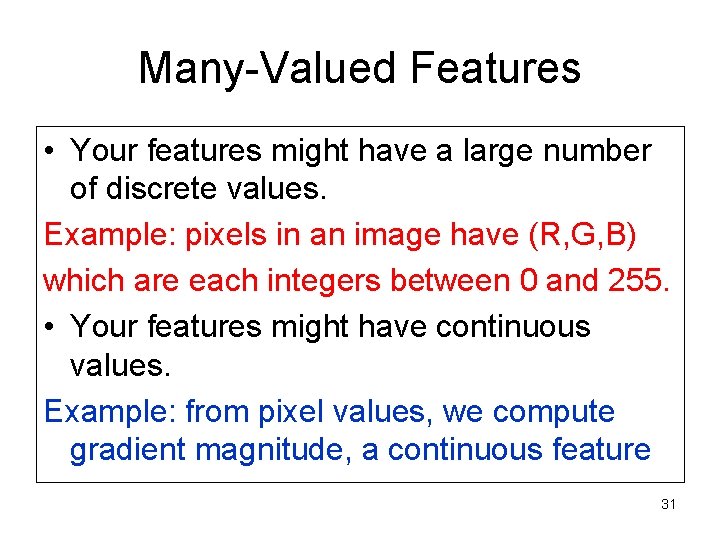
feature vector (square, red) (square, blue) (circle, red) (circle blue) (triangle, red) (triangle, green) (ellipse, blue) (ellipse, red) class I I II II Try the color feature I I II II red Entropy? blue green Entropy? GAIN? 30

Many-Valued Features • Your features might have a large number of discrete values. Example: pixels in an image have (R, G, B) which are each integers between 0 and 255. • Your features might have continuous values. Example: from pixel values, we compute gradient magnitude, a continuous feature 31

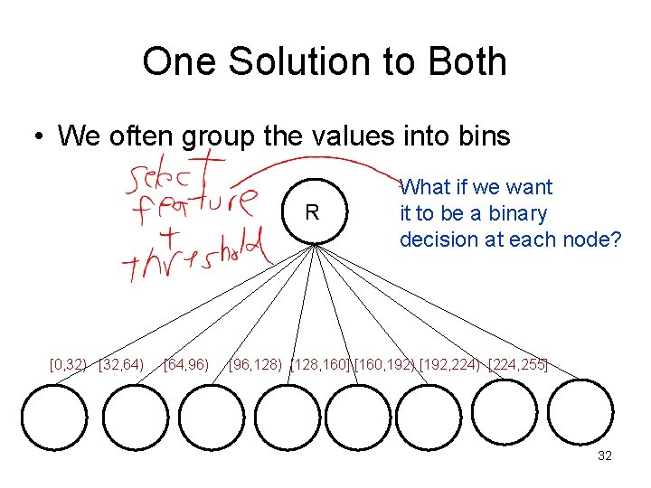
One Solution to Both • We often group the values into bins R [0, 32) [32, 64) [64, 96) What if we want it to be a binary decision at each node? [96, 128) [128, 160] [160, 192) [192, 224) [224, 255] 32

Training and Testing • Divide data into a training set and a separate testing set. • Construct the decision tree using the training set only. • Test the decision tree on the training set to see how it’s doing. • Test the decision tree on the testing set to report its real performance. 33

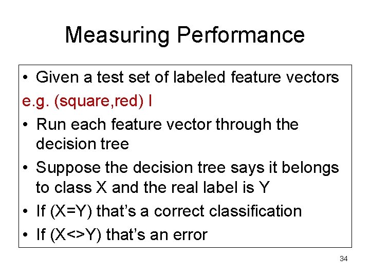
Measuring Performance • Given a test set of labeled feature vectors e. g. (square, red) I • Run each feature vector through the decision tree • Suppose the decision tree says it belongs to class X and the real label is Y • If (X=Y) that’s a correct classification • If (X<>Y) that’s an error 34

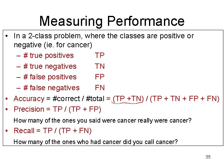
Measuring Performance • In a 2 -class problem, where the classes are positive or negative (ie. for cancer) – # true positives TP – # true negatives TN – # false positives FP – # false negatives FN • Accuracy = #correct / #total = (TP +TN) / (TP + TN + FP + FN) • Precision = TP / (TP + FP) How many of the ones you said were cancer really were cancer? • Recall = TP / (TP + FN) How many of the ones who had cancer did you call cancer? 35

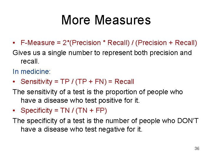
More Measures • F-Measure = 2*(Precision * Recall) / (Precision + Recall) Gives us a single number to represent both precision and recall. In medicine: • Sensitivity = TP / (TP + FN) = Recall The sensitivity of a test is the proportion of people who have a disease who test positive for it. • Specificity = TN / (TN + FP) The specificity of a test is the number of people who DON’T have a disease who test negative for it. 36

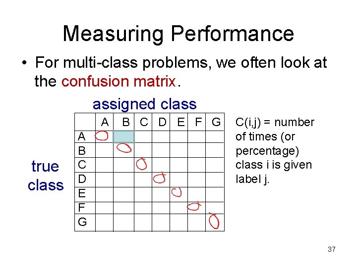
Measuring Performance • For multi-class problems, we often look at the confusion matrix. assigned class A true class A B C D E F G C(i, j) = number of times (or percentage) class i is given label j. 37

Overfitting • Suppose the classifier h has error (1 accuracy) of errortrain(h) • And there is an alternate classifier (hypothesis) h’ that has errortrain(h’) • What if errortrain(h) < errortrain(h’) • But error. D(h) > error. D(h’) for full set D • Then we say h overfits the training data 38

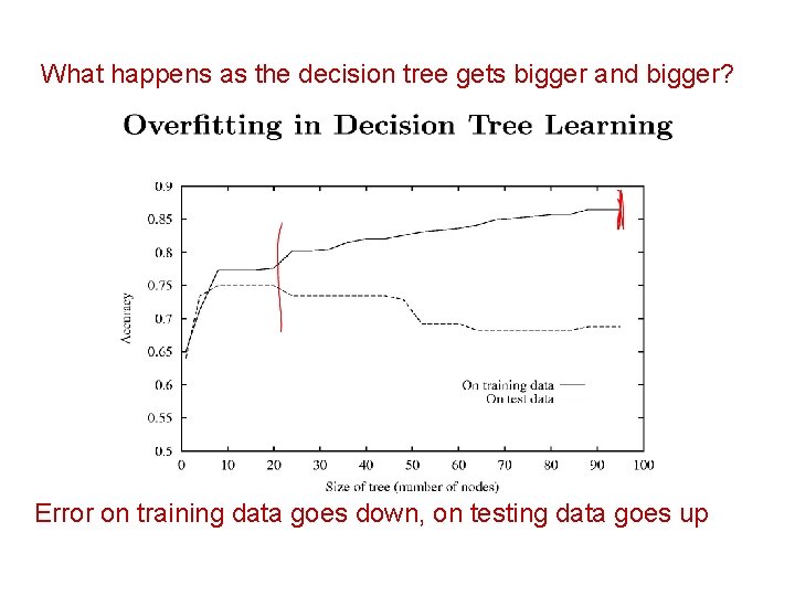
What happens as the decision tree gets bigger and bigger? Error on training data goes down, on testing data goes up 39

Reduced Error Pruning • Split data into training and validation sets • Do until further pruning is harmful 1. Evaluate impact on validation set of pruning each possible node (and its subtree) 2. Greedily remove the one that most improves validation set accuracy • Then you need an additional independent testing set. 40

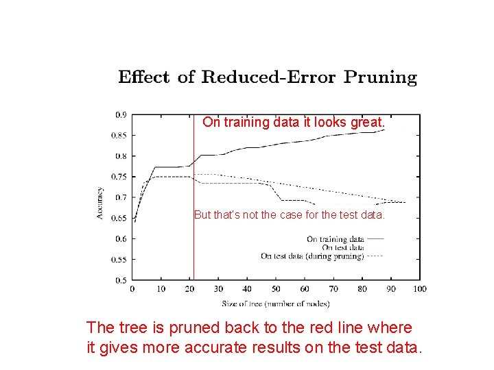
On training data it looks great. But that’s not the case for the test data. The tree is pruned back to the red line where it gives more accurate results on the test data. 41

• The WEKA example with Calenouria and Dorenouria I showed you used the REPTree classifier with 21 nodes. • The classic decision tree for the same data had 65 nodes. • Performance was similar for our test set. • Performance increased using a random forest of 10 trees, each constructed with 7 random features. 42

Decision Trees: Summary • Representation=decision trees • Bias=preference for small decision trees • Search algorithm=none • Heuristic function=information gain or information content or others • Overfitting and pruning • Advantage is simplicity and easy conversion to rules. 43

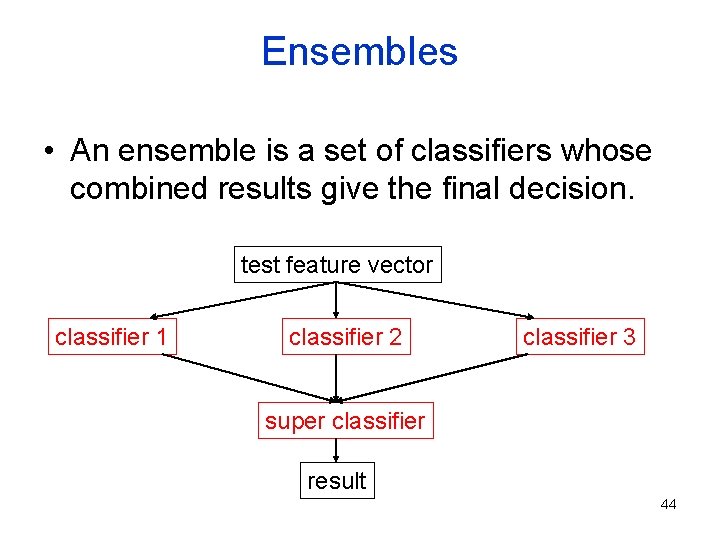
Ensembles • An ensemble is a set of classifiers whose combined results give the final decision. test feature vector classifier 1 classifier 2 classifier 3 super classifier result 44

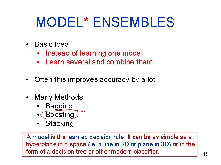
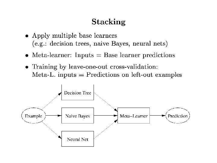
MODEL* ENSEMBLES • Basic Idea • Instead of learning one model • Learn several and combine them • Often this improves accuracy by a lot • Many Methods • Bagging • Boosting • Stacking *A model is the learned decision rule. It can be as simple as a hyperplane in n-space (ie. a line in 2 D or plane in 3 D) or in the form of a decision tree or other modern classifier. 45

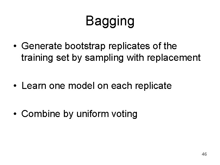
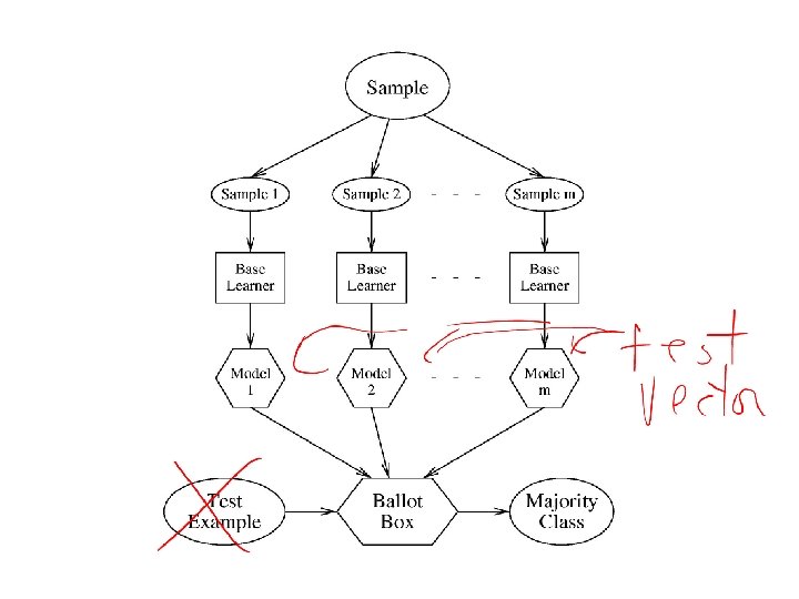
Bagging • Generate bootstrap replicates of the training set by sampling with replacement • Learn one model on each replicate • Combine by uniform voting 46

47

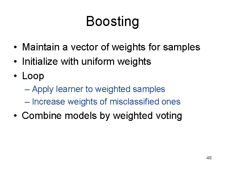
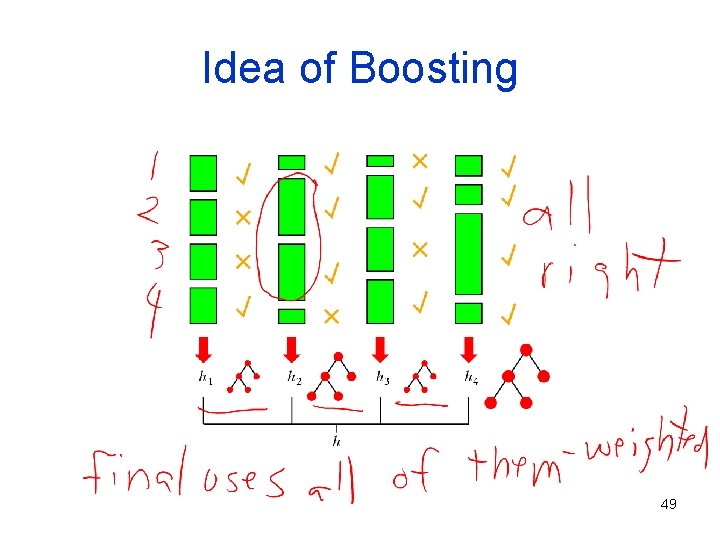
Boosting • Maintain a vector of weights for samples • Initialize with uniform weights • Loop – Apply learner to weighted samples – Increase weights of misclassified ones • Combine models by weighted voting 48

Idea of Boosting 49

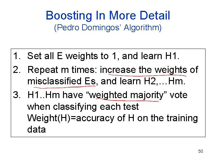
Boosting In More Detail (Pedro Domingos’ Algorithm) 1. Set all E weights to 1, and learn H 1. 2. Repeat m times: increase the weights of misclassified Es, and learn H 2, …Hm. 3. H 1. . Hm have “weighted majority” vote when classifying each test Weight(H)=accuracy of H on the training data 50

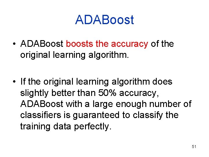
ADABoost • ADABoost boosts the accuracy of the original learning algorithm. • If the original learning algorithm does slightly better than 50% accuracy, ADABoost with a large enough number of classifiers is guaranteed to classify the training data perfectly. 51

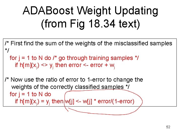
ADABoost Weight Updating (from Fig 18. 34 text) /* First find the sum of the weights of the misclassified samples */ for j = 1 to N do /* go through training samples */ if h[m](xj) <> yj then error <- error + wj /* Now use the ratio of error to 1 -error to change the weights of the correctly classified samples */ for j = 1 to N do if h[m](xj) = yj then w[j] <- w[j] * error/(1 -error) 52

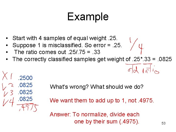
Example • Start with 4 samples of equal weight. 25. • Suppose 1 is misclassified. So error =. 25. • The ratio comes out. 25/. 75 =. 33 • The correctly classified samples get weight of. 25*. 33 =. 0825. 2500. 0825 What’s wrong? What should we do? We want them to add up to 1, not. 4975. Answer: To normalize, divide each one by their sum (. 4975). 53

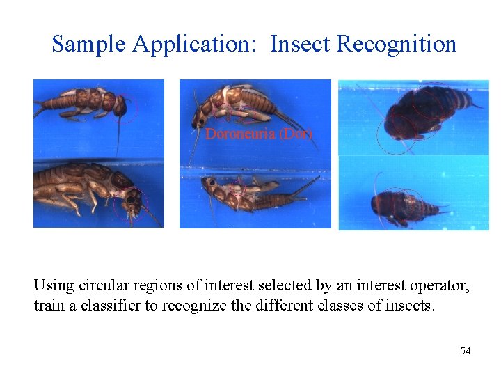
Sample Application: Insect Recognition Doroneuria (Dor) Using circular regions of interest selected by an interest operator, train a classifier to recognize the different classes of insects. 54

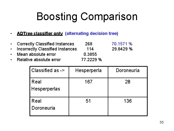
Boosting Comparison • ADTree classifier only (alternating decision tree) • • Correctly Classified Instances 268 Incorrectly Classified Instances 114 Mean absolute error 0. 3855 Relative absolute error 77. 2229 % Classified as -> 70. 1571 % 29. 8429 % Hesperperla Doroneuria Real Hesperperlas 167 28 Real Doroneuria 51 136 55

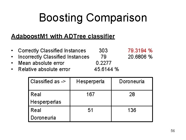
Boosting Comparison Adaboost. M 1 with ADTree classifier • • Correctly Classified Instances 303 Incorrectly Classified Instances 79 Mean absolute error 0. 2277 Relative absolute error 45. 6144 % Classified as -> 79. 3194 % 20. 6806 % Hesperperla Doroneuria Real Hesperperlas 167 28 Real Doroneuria 51 136 56

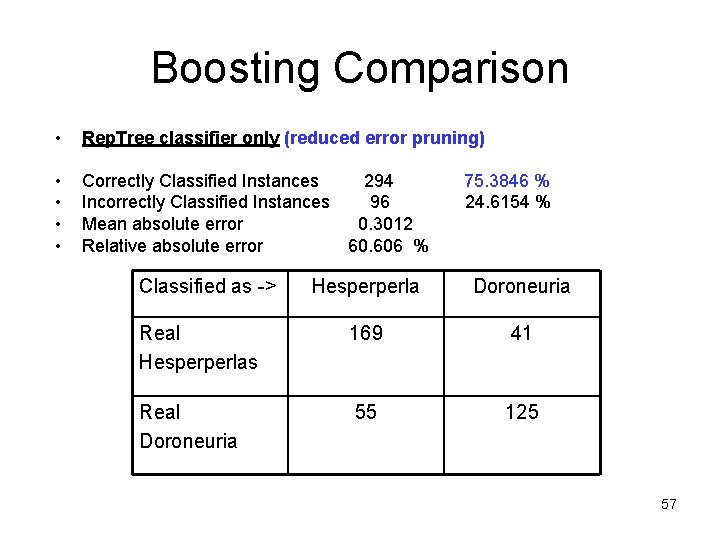
Boosting Comparison • Rep. Tree classifier only (reduced error pruning) • • Correctly Classified Instances 294 Incorrectly Classified Instances 96 Mean absolute error 0. 3012 Relative absolute error 60. 606 % Classified as -> 75. 3846 % 24. 6154 % Hesperperla Doroneuria Real Hesperperlas 169 41 Real Doroneuria 55 125 57

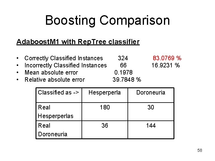
Boosting Comparison Adaboost. M 1 with Rep. Tree classifier • • Correctly Classified Instances 324 Incorrectly Classified Instances 66 Mean absolute error 0. 1978 Relative absolute error 39. 7848 % Classified as -> 83. 0769 % 16. 9231 % Hesperperla Doroneuria Real Hesperperlas 180 30 Real Doroneuria 36 144 58

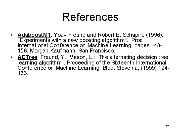
References • Adaboost. M 1: Yoav Freund and Robert E. Schapire (1996). "Experiments with a new boosting algorithm". Proc International Conference on Machine Learning, pages 148156, Morgan Kaufmann, San Francisco. • ADTree: Freund, Y. , Mason, L. : "The alternating decision tree learning algorithm". Proceeding of the Sixteenth International Conference on Machine Learning, Bled, Slovenia, (1999) 124133. 59

60

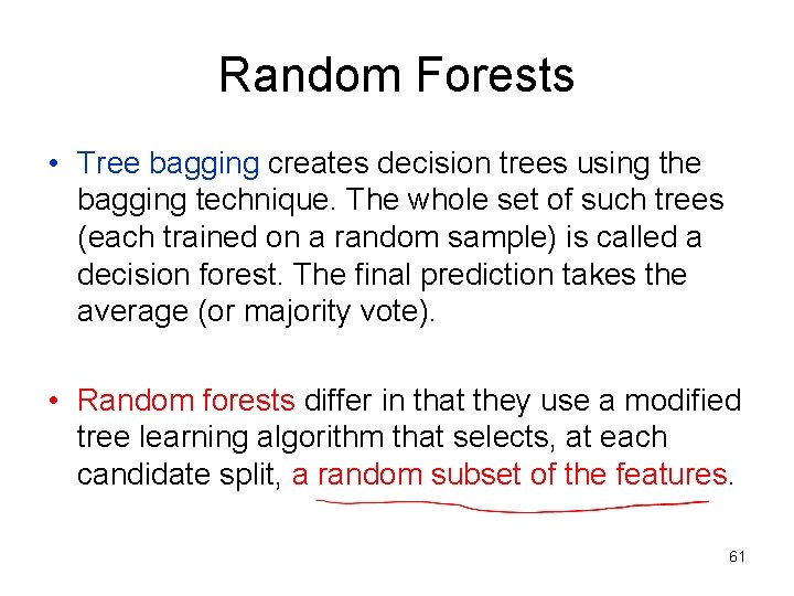
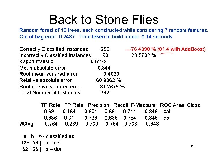
Random Forests • Tree bagging creates decision trees using the bagging technique. The whole set of such trees (each trained on a random sample) is called a decision forest. The final prediction takes the average (or majority vote). • Random forests differ in that they use a modified tree learning algorithm that selects, at each candidate split, a random subset of the features. 61

Back to Stone Flies Random forest of 10 trees, each constructed while considering 7 random features. Out of bag error: 0. 2487. Time taken to build model: 0. 14 seconds Correctly Classified Instances 292 Incorrectly Classified Instances 90 Kappa statistic 0. 5272 Mean absolute error 0. 344 Root mean squared error 0. 4069 Relative absolute error 68. 9062 % Root relative squared error 81. 2679 % Total Number of Instances 382 WAvg. TP Rate 0. 69 0. 836 0. 764 76. 4398 % (81. 4 with Ada. Boost) 23. 5602 % FP Rate Precision Recall F-Measure ROC Area Class 0. 164 0. 801 0. 69 0. 741 0. 848 cal 0. 31 0. 738 0. 836 0. 784 0. 848 dor 0. 239 0. 764 0. 763 0. 848 a b <-- classified as 129 58 | a = cal 32 163 | b = dor 62