CS 179 GPU Programming Lecture 10 Topics Nonnumerical

CS 179: GPU Programming Lecture 10

Topics • Non-numerical algorithms – Parallel breadth-first search (BFS) • Texture memory

• GPUs – good for many numerical calculations… • What about “non-numerical” problems?

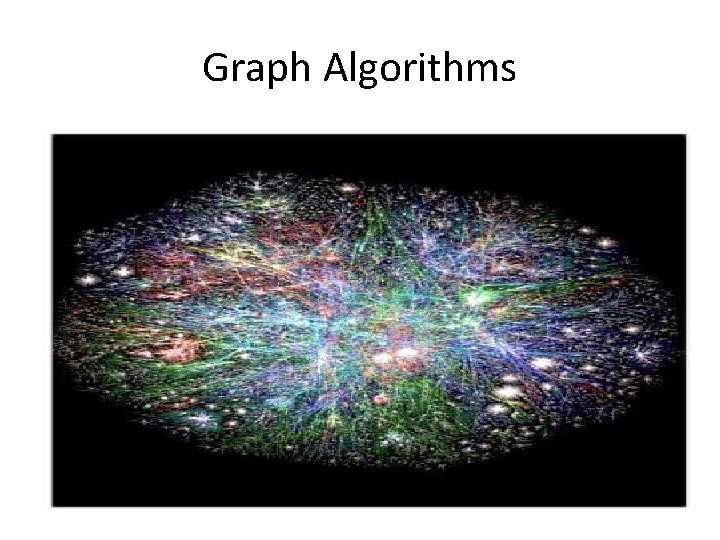
Graph Algorithms

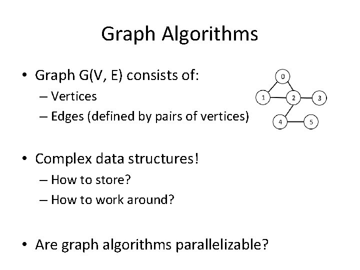
Graph Algorithms • Graph G(V, E) consists of: – Vertices – Edges (defined by pairs of vertices) • Complex data structures! – How to store? – How to work around? • Are graph algorithms parallelizable?

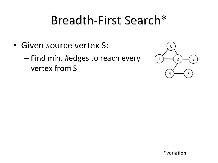
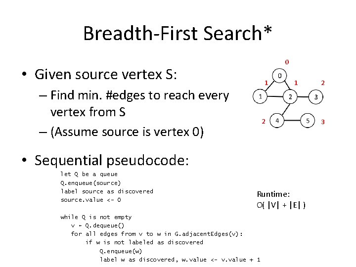
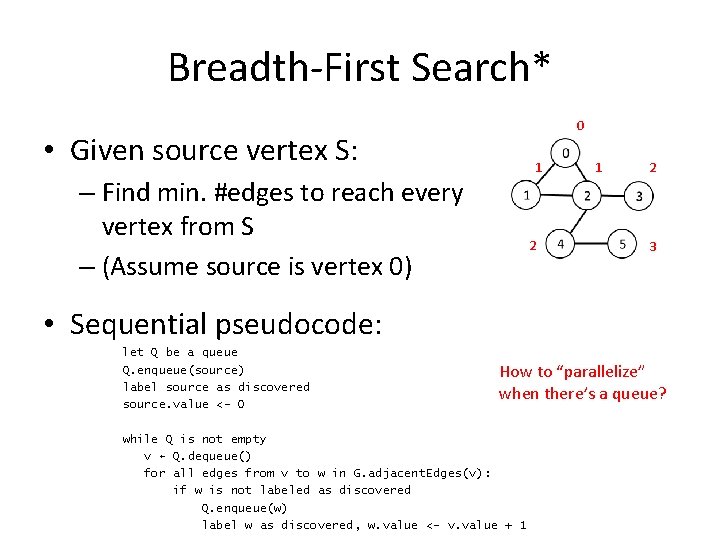
Breadth-First Search* • Given source vertex S: – Find min. #edges to reach every vertex from S *variation

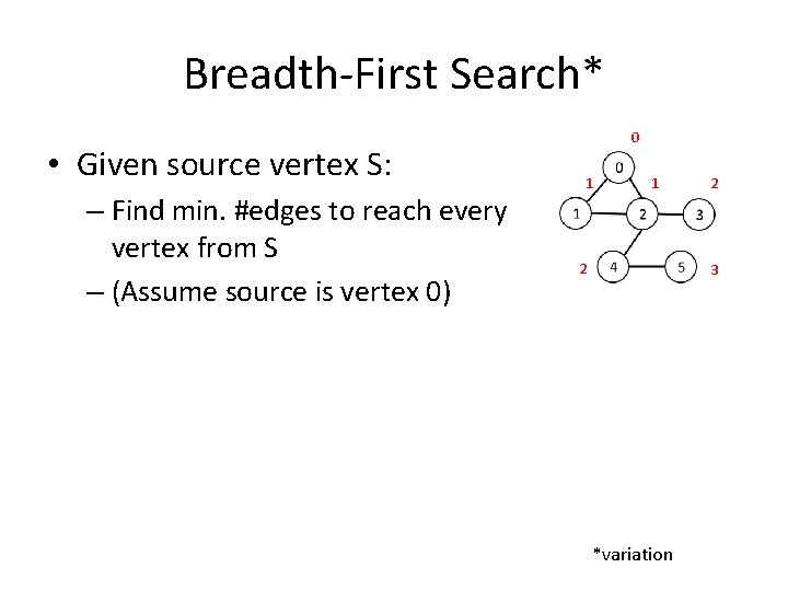
Breadth-First Search* • Given source vertex S: – Find min. #edges to reach every vertex from S – (Assume source is vertex 0) 0 1 1 2 2 3 *variation

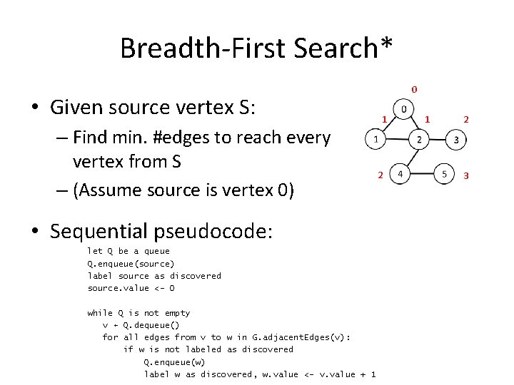
Breadth-First Search* • Given source vertex S: – Find min. #edges to reach every vertex from S – (Assume source is vertex 0) • Sequential pseudocode: let Q be a queue Q. enqueue(source) label source as discovered source. value <- 0 while Q is not empty v ← Q. dequeue() for all edges from v to w in G. adjacent. Edges(v): if w is not labeled as discovered Q. enqueue(w) label w as discovered, w. value <- v. value + 1 0 1 2 3

Breadth-First Search* 0 • Given source vertex S: 1 – Find min. #edges to reach every vertex from S – (Assume source is vertex 0) 1 2 • Sequential pseudocode: let Q be a queue Q. enqueue(source) label source as discovered source. value <- 0 Runtime: O( |V| + |E| ) while Q is not empty v ← Q. dequeue() for all edges from v to w in G. adjacent. Edges(v): if w is not labeled as discovered Q. enqueue(w) label w as discovered, w. value <- v. value + 1 2 3

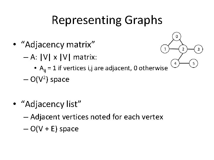
Representing Graphs • “Adjacency matrix” – A: |V| x |V| matrix: • Aij = 1 if vertices i, j are adjacent, 0 otherwise – O(V 2) space • “Adjacency list” – Adjacent vertices noted for each vertex – O(V + E) space

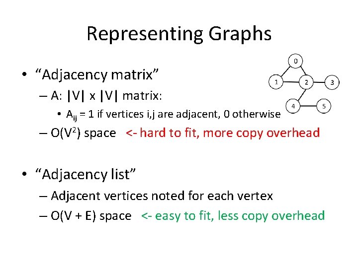
Representing Graphs • “Adjacency matrix” – A: |V| x |V| matrix: • Aij = 1 if vertices i, j are adjacent, 0 otherwise – O(V 2) space <- hard to fit, more copy overhead • “Adjacency list” – Adjacent vertices noted for each vertex – O(V + E) space <- easy to fit, less copy overhead

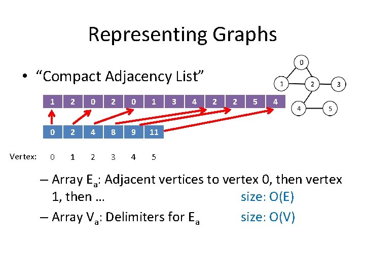
Representing Graphs • “Compact Adjacency List” Vertex: 1 2 0 1 0 2 4 8 9 11 0 1 2 3 4 5 3 4 2 2 5 4 – Array Ea: Adjacent vertices to vertex 0, then vertex 1, then … size: O(E) – Array Va: Delimiters for Ea size: O(V)

Breadth-First Search* 0 • Given source vertex S: 1 – Find min. #edges to reach every vertex from S – (Assume source is vertex 0) 2 1 2 3 • Sequential pseudocode: let Q be a queue Q. enqueue(source) label source as discovered source. value <- 0 How to “parallelize” when there’s a queue? while Q is not empty v ← Q. dequeue() for all edges from v to w in G. adjacent. Edges(v): if w is not labeled as discovered Q. enqueue(w) label w as discovered, w. value <- v. value + 1

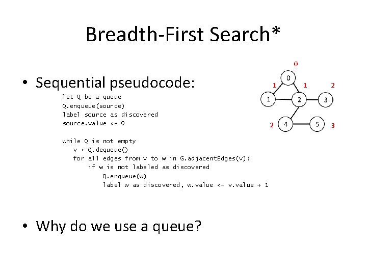
Breadth-First Search* 0 • Sequential pseudocode: let Q be a queue Q. enqueue(source) label source as discovered source. value <- 0 while Q is not empty v ← Q. dequeue() for all edges from v to w in G. adjacent. Edges(v): if w is not labeled as discovered Q. enqueue(w) label w as discovered, w. value <- v. value + 1 • Why do we use a queue? 1 2 3

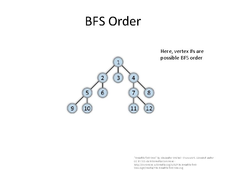
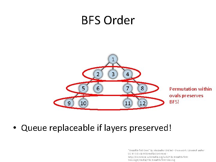
BFS Order Here, vertex #s are possible BFS order "Breadth-first-tree" by Alexander Drichel - Own work. Licensed under CC BY 3. 0 via Wikimedia Commons http: //commons. wikimedia. org/wiki/File: Breadth-firsttree. svg#/media/File: Breadth-first-tree. svg

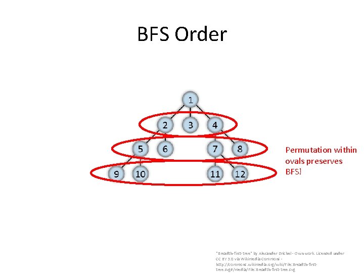
BFS Order Permutation within ovals preserves BFS! "Breadth-first-tree" by Alexander Drichel - Own work. Licensed under CC BY 3. 0 via Wikimedia Commons http: //commons. wikimedia. org/wiki/File: Breadth-firsttree. svg#/media/File: Breadth-first-tree. svg

BFS Order Permutation within ovals preserves BFS! • Queue replaceable if layers preserved! "Breadth-first-tree" by Alexander Drichel - Own work. Licensed under CC BY 3. 0 via Wikimedia Commons http: //commons. wikimedia. org/wiki/File: Breadth-firsttree. svg#/media/File: Breadth-first-tree. svg

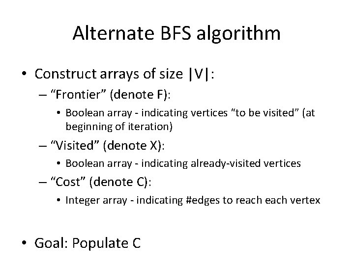
Alternate BFS algorithm • Construct arrays of size |V|: – “Frontier” (denote F): • Boolean array - indicating vertices “to be visited” (at beginning of iteration) – “Visited” (denote X): • Boolean array - indicating already-visited vertices – “Cost” (denote C): • Integer array - indicating #edges to reach vertex • Goal: Populate C

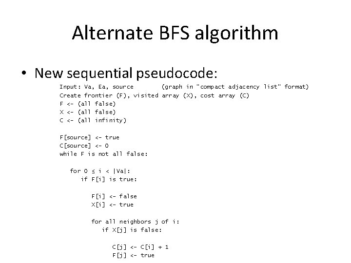
Alternate BFS algorithm • New sequential pseudocode: Input: Va, Ea, source (graph in “compact adjacency list” format) Create frontier (F), visited array (X), cost array (C) F <- (all false) X <- (all false) C <- (all infinity) F[source] <- true C[source] <- 0 while F is not all false: for 0 ≤ i < |Va|: if F[i] is true: F[i] <- false X[i] <- true for all neighbors j of i: if X[j] is false: C[j] <- C[i] + 1 F[j] <- true

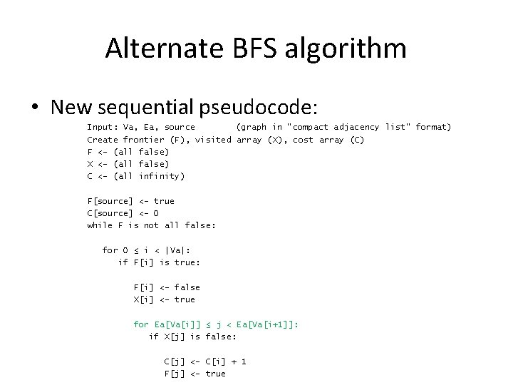
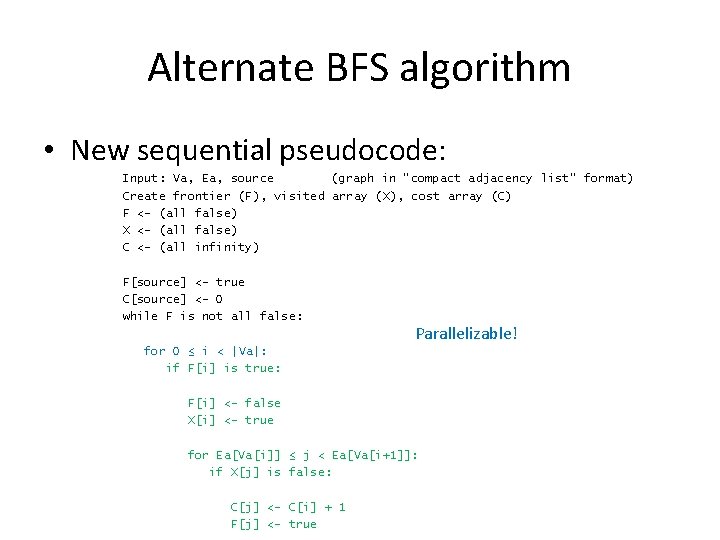
Alternate BFS algorithm • New sequential pseudocode: Input: Va, Ea, source (graph in “compact adjacency list” format) Create frontier (F), visited array (X), cost array (C) F <- (all false) X <- (all false) C <- (all infinity) F[source] <- true C[source] <- 0 while F is not all false: for 0 ≤ i < |Va|: if F[i] is true: F[i] <- false X[i] <- true for Ea[Va[i]] ≤ j < Ea[Va[i+1]]: if X[j] is false: C[j] <- C[i] + 1 F[j] <- true

Alternate BFS algorithm • New sequential pseudocode: Input: Va, Ea, source (graph in “compact adjacency list” format) Create frontier (F), visited array (X), cost array (C) F <- (all false) X <- (all false) C <- (all infinity) F[source] <- true C[source] <- 0 while F is not all false: Parallelizable! for 0 ≤ i < |Va|: if F[i] is true: F[i] <- false X[i] <- true for Ea[Va[i]] ≤ j < Ea[Va[i+1]]: if X[j] is false: C[j] <- C[i] + 1 F[j] <- true

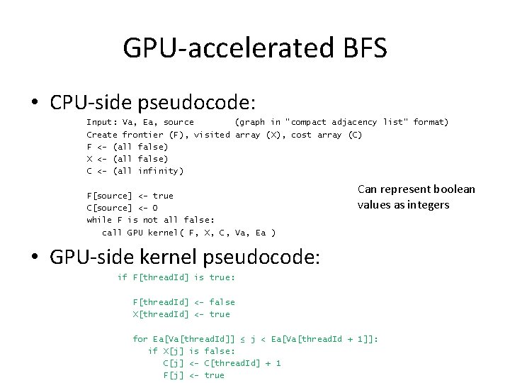
GPU-accelerated BFS • CPU-side pseudocode: Input: Va, Ea, source (graph in “compact adjacency list” format) Create frontier (F), visited array (X), cost array (C) F <- (all false) X <- (all false) C <- (all infinity) F[source] <- true C[source] <- 0 while F is not all false: call GPU kernel( F, X, C, Va, Ea ) Can represent boolean values as integers • GPU-side kernel pseudocode: if F[thread. Id] is true: F[thread. Id] <- false X[thread. Id] <- true for Ea[Va[thread. Id]] ≤ j < Ea[Va[thread. Id + 1]]: if X[j] is false: C[j] <- C[thread. Id] + 1 F[j] <- true

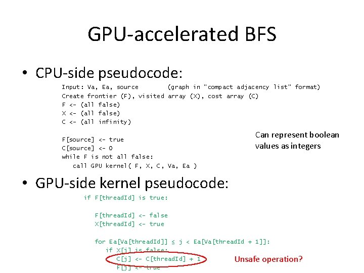
GPU-accelerated BFS • CPU-side pseudocode: Input: Va, Ea, source (graph in “compact adjacency list” format) Create frontier (F), visited array (X), cost array (C) F <- (all false) X <- (all false) C <- (all infinity) F[source] <- true C[source] <- 0 while F is not all false: call GPU kernel( F, X, C, Va, Ea ) Can represent boolean values as integers • GPU-side kernel pseudocode: if F[thread. Id] is true: F[thread. Id] <- false X[thread. Id] <- true for Ea[Va[thread. Id]] ≤ j < Ea[Va[thread. Id + 1]]: if X[j] is false: C[j] <- C[thread. Id] + 1 Unsafe operation? F[j] <- true

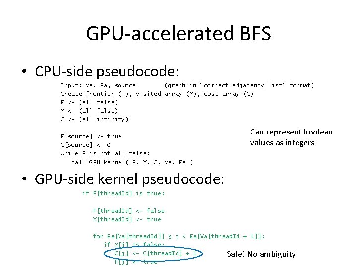
GPU-accelerated BFS • CPU-side pseudocode: Input: Va, Ea, source (graph in “compact adjacency list” format) Create frontier (F), visited array (X), cost array (C) F <- (all false) X <- (all false) C <- (all infinity) F[source] <- true C[source] <- 0 while F is not all false: call GPU kernel( F, X, C, Va, Ea ) Can represent boolean values as integers • GPU-side kernel pseudocode: if F[thread. Id] is true: F[thread. Id] <- false X[thread. Id] <- true for Ea[Va[thread. Id]] ≤ j < Ea[Va[thread. Id + 1]]: if X[j] is false: C[j] <- C[thread. Id] + 1 Safe! No ambiguity! F[j] <- true

Summary • Tricky algorithms need drastic measures! • Resources – “Accelerating Large Graph Algorithms on the GPU Using CUDA” (Harish, Narayanan)

Texture Memory

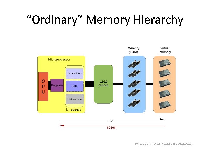
“Ordinary” Memory Hierarchy http: //www. imm. dtu. dk/~beda/Sci. Comp/caches. png

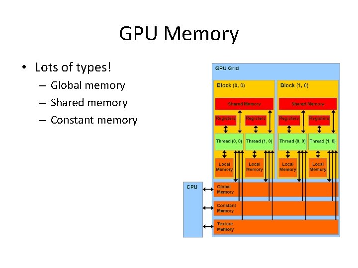
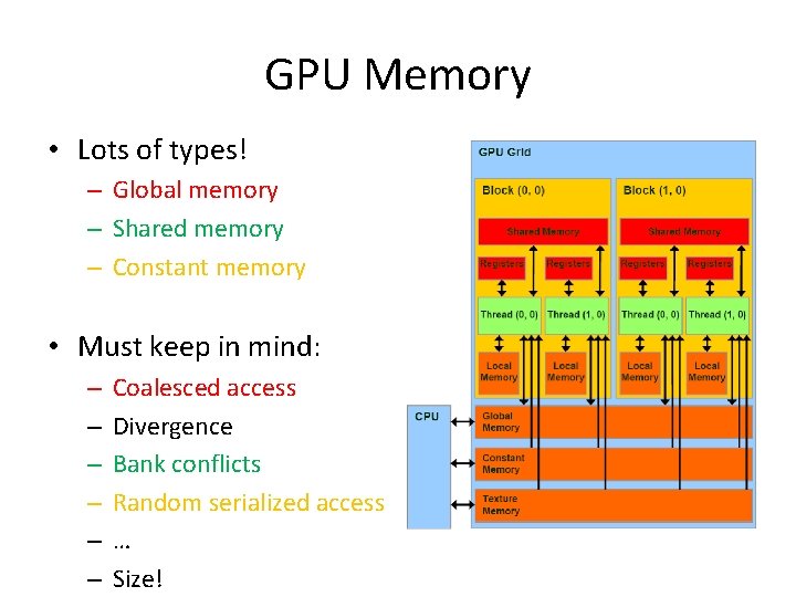
GPU Memory • Lots of types! – Global memory – Shared memory – Constant memory

GPU Memory • Lots of types! – Global memory – Shared memory – Constant memory • Must keep in mind: – – – Coalesced access Divergence Bank conflicts Random serialized access … Size!

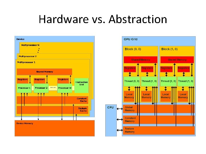
Hardware vs. Abstraction

Hardware vs. Abstraction • Names refer to manner of access on device memory: – “Global memory” – “Constant memory” – “Texture memory”

Review: Constant Memory • Read-only access • 64 KB available, 8 KB cache – small! • Not “const”! – Write to region with cuda. Memcpy. To. Symbol()

Review: Constant Memory • Broadcast reads to half-warps! – When all threads need same data: Save reads! • Downside: – When all threads need different data: Extremely slow!

Review: Constant Memory • Example application: Gaussian impulse response (from HW 1): – Not changed – Accessed simultaneously by threads in warp

Texture Memory (and co-stars) • Another type of memory system, featuring: – Spatially-cached read-only access – Avoid coalescing worries – Interpolation – (Other) fixed-function capabilities – Graphics interoperability

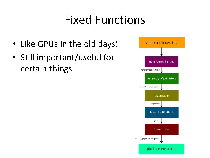
Fixed Functions • Like GPUs in the old days! • Still important/useful for certain things

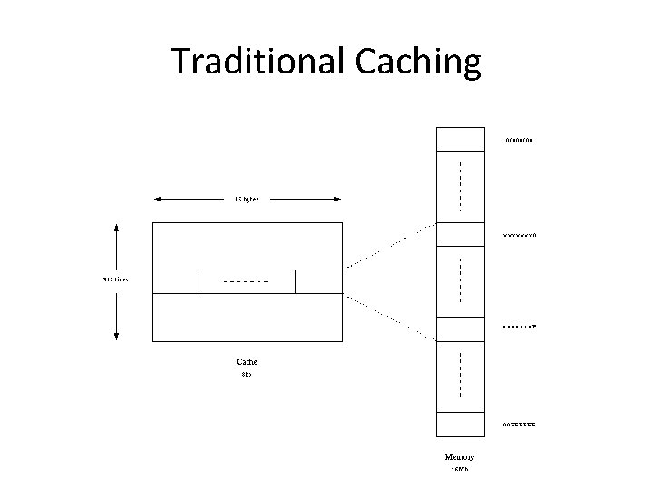
Traditional Caching • When reading, cache “nearby elements” – (i. e. cache line) – Memory is linear! – Applies to CPU, GPU L 1/L 2 cache, etc

Traditional Caching

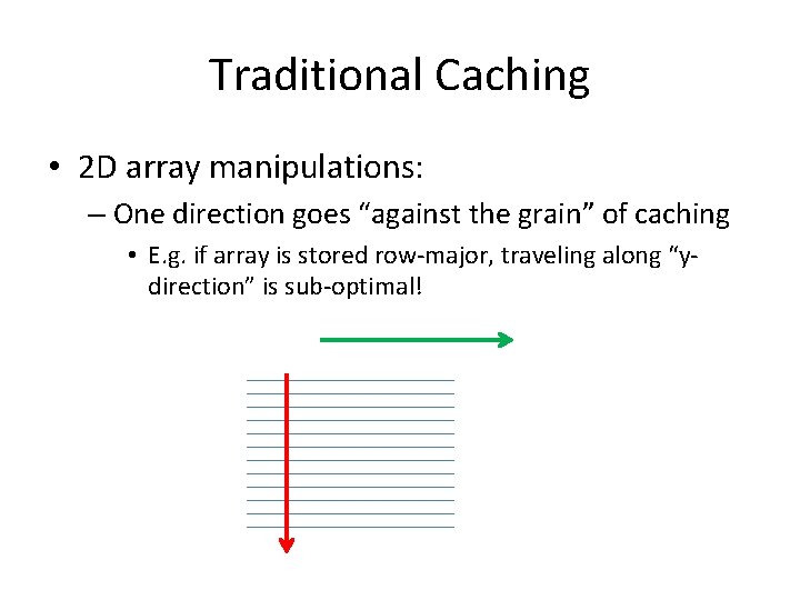
Traditional Caching • 2 D array manipulations: – One direction goes “against the grain” of caching • E. g. if array is stored row-major, traveling along “ydirection” is sub-optimal!

Texture-Memory Caching • Can cache “spatially!” (2 D, 3 D) – Specify dimensions (1 D, 2 D, 3 D) on creation • 1 D applications: – Interpolation, clipping (later) – Caching when e. g. coalesced access is infeasible

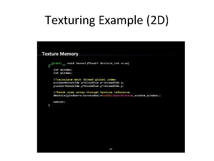
Texture Memory • “Memory is just an unshaped bucket of bits” (CUDA Handbook) • Need texture reference in order to: – Interpret data – Deliver to registers

Texture References • “Bound” to regions of memory • Specify (depending on situation): – Access dimensions (1 D, 2 D, 3 D) – Interpolation behavior – “Clamping” behavior – Normalization –…

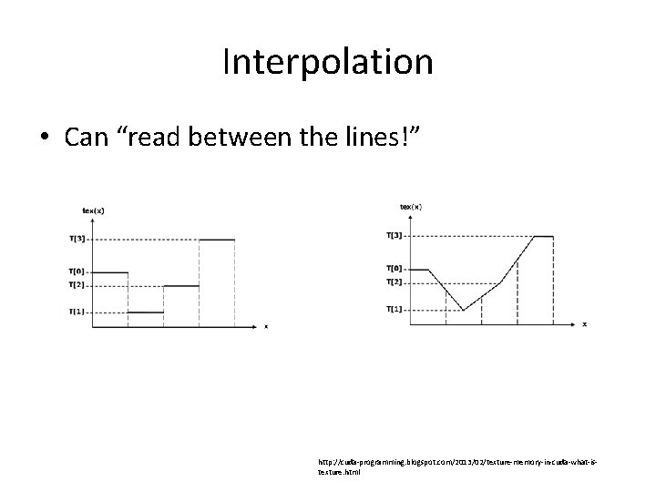
Interpolation • Can “read between the lines!” http: //cuda-programming. blogspot. com/2013/02/texture-memory-in-cuda-what-istexture. html

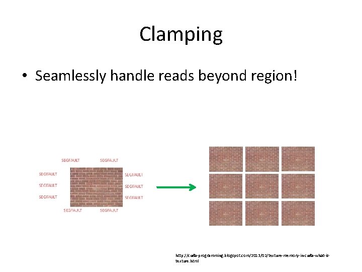
Clamping • Seamlessly handle reads beyond region! http: //cuda-programming. blogspot. com/2013/02/texture-memory-in-cuda-what-istexture. html

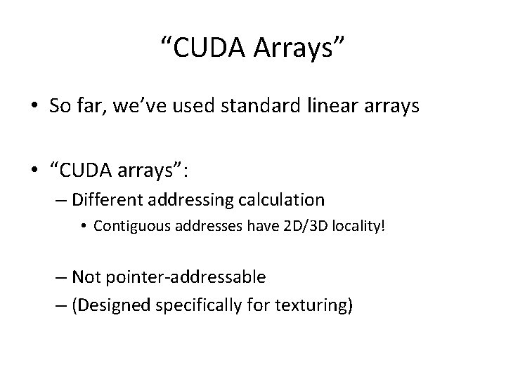
“CUDA Arrays” • So far, we’ve used standard linear arrays • “CUDA arrays”: – Different addressing calculation • Contiguous addresses have 2 D/3 D locality! – Not pointer-addressable – (Designed specifically for texturing)

Texture Memory • Texture reference can be attached to: – Ordinary device-memory array – “CUDA array” • Many more capabilities

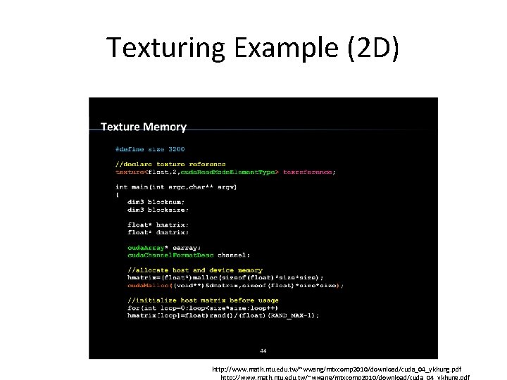
Texturing Example (2 D) http: //www. math. ntu. edu. tw/~wwang/mtxcomp 2010/download/cuda_04_ykhung. pdf

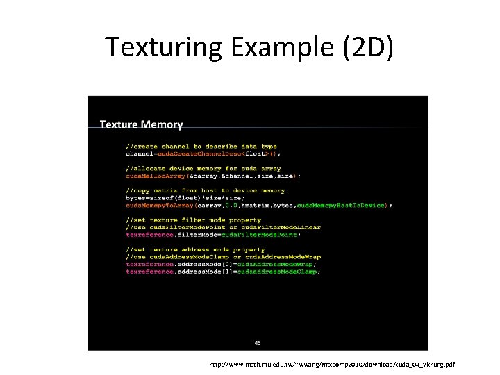
Texturing Example (2 D) http: //www. math. ntu. edu. tw/~wwang/mtxcomp 2010/download/cuda_04_ykhung. pdf

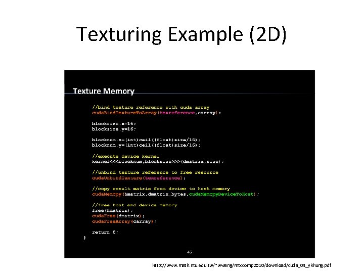
Texturing Example (2 D) http: //www. math. ntu. edu. tw/~wwang/mtxcomp 2010/download/cuda_04_ykhung. pdf

Texturing Example (2 D)