CS 179 GPU Programming Lecture 8 Last time

CS 179: GPU Programming Lecture 8

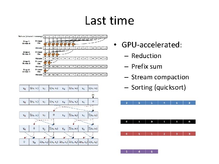
Last time • GPU-accelerated: – – Reduction Prefix sum Stream compaction Sorting (quicksort)

Today • GPU-accelerated Fast Fourier Transform • cu. FFT (FFT library) • This lecture – details behind FFT algorithm. Shows why you shouldn’t re-invent the wheel! – Don’t implement what a library already does for you, if you don’t have to! • It’s not TOO critical for the HW for many of the details about this math – mostly background. • We will use this FFT in the final weeks of lecture before projects, for implementing CONVOLUTIONAL NETWORKS on GPUs.

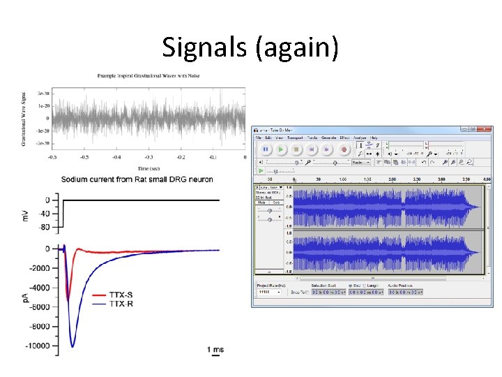
Signals (again)

“Frequency content” • FT answers question: “What frequencies are present in our signals? ” • Key to field of Digital Signal Processing -- see https: //en. wikipedia. org/wiki/Digital_signal_processing • Time domain – higher frequencies are higher pitch • Spatial domain – works similarly, but with “x” instead of “t”

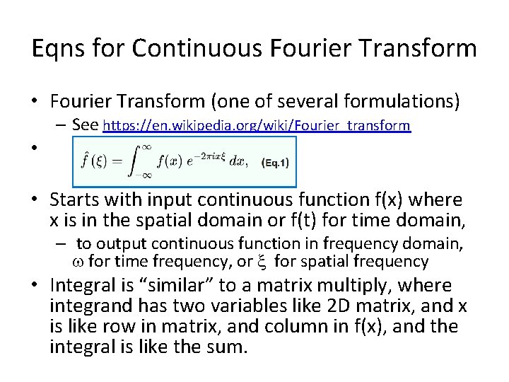
Eqns for Continuous Fourier Transform • Fourier Transform (one of several formulations) – See https: //en. wikipedia. org/wiki/Fourier_transform • • Starts with input continuous function f(x) where x is in the spatial domain or f(t) for time domain, – to output continuous function in frequency domain, w for time frequency, or x for spatial frequency • Integral is “similar” to a matrix multiply, where integrand has two variables like 2 D matrix, and x is like row in matrix, and column in f(x), and the integral is like the sum.

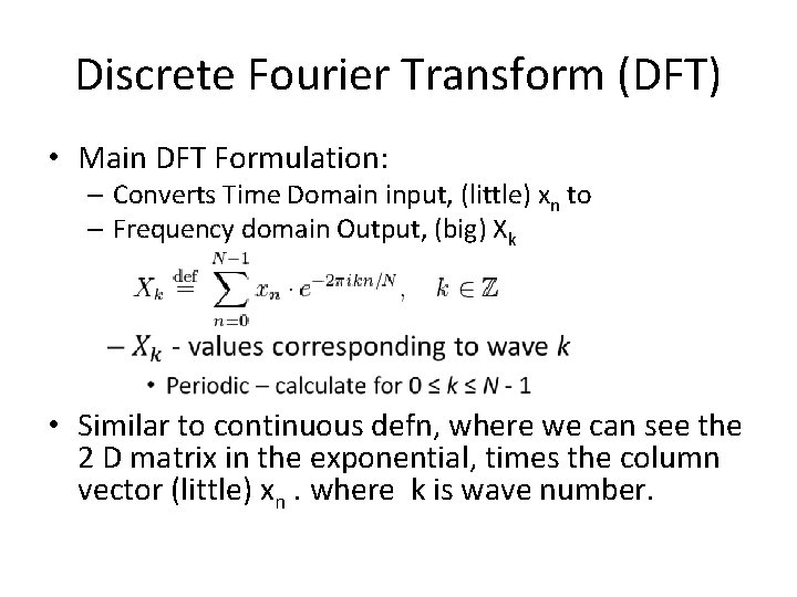
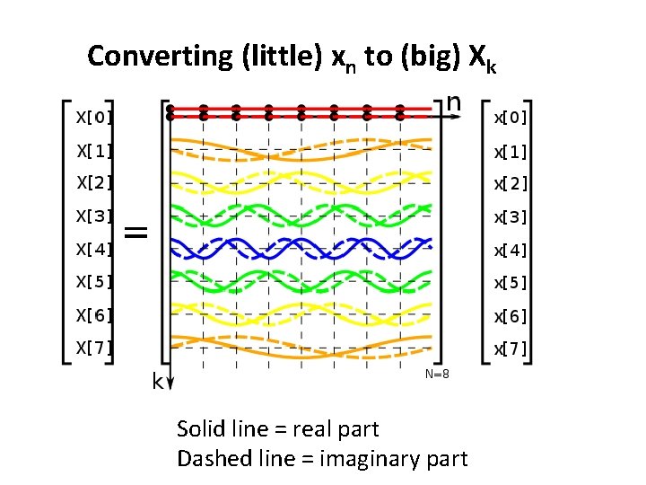
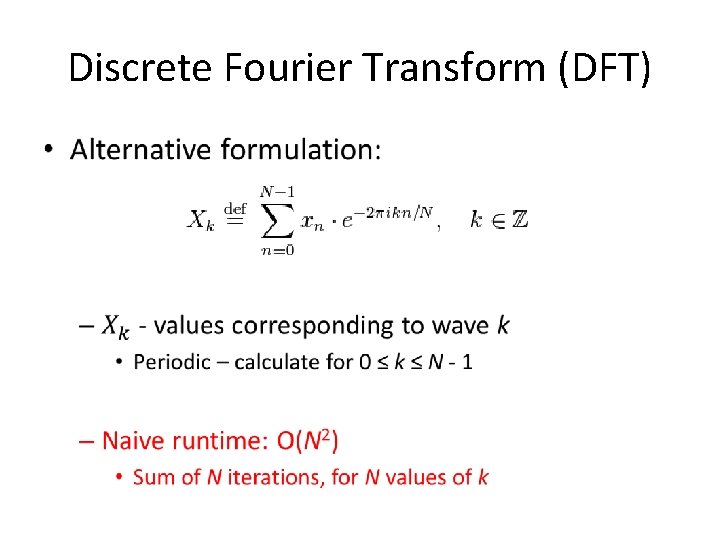
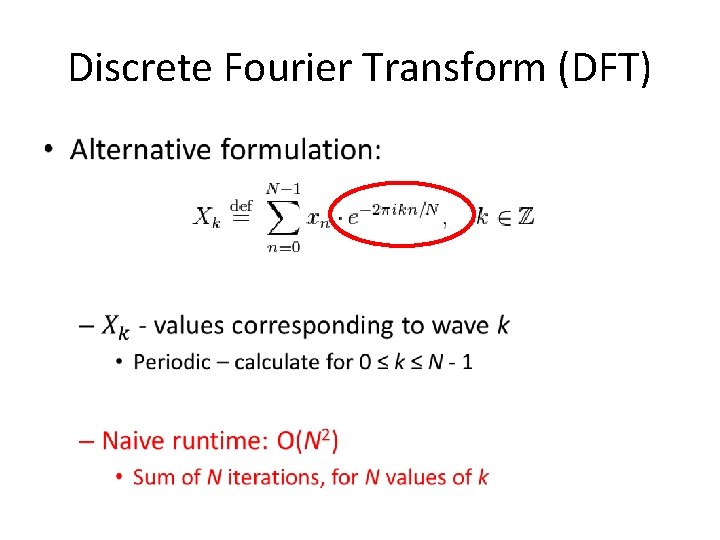
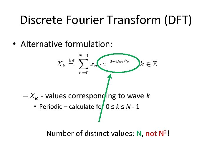
Discrete Fourier Transform (DFT) • Main DFT Formulation: – Converts Time Domain input, (little) xn to – Frequency domain Output, (big) Xk • Similar to continuous defn, where we can see the 2 D matrix in the exponential, times the column vector (little) xn. where k is wave number.

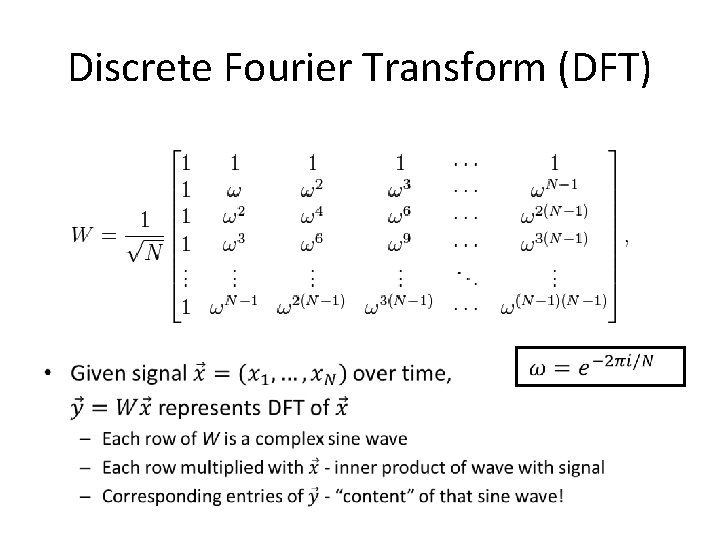
Discrete Fourier Transform (DFT) •

Converting (little) xn to (big) Xk Solid line = real part Dashed line = imaginary part

Discrete Fourier Transform (DFT) •

Discrete Fourier Transform (DFT) •

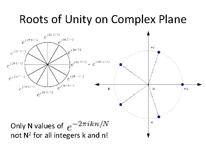
Roots of Unity on Complex Plane Only N values of not N 2 for all integers k and n!

Discrete Fourier Transform (DFT) • Number of distinct values: N, not N 2!

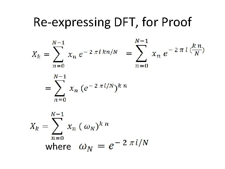
Re-expressing DFT, for Proof where

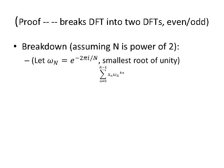
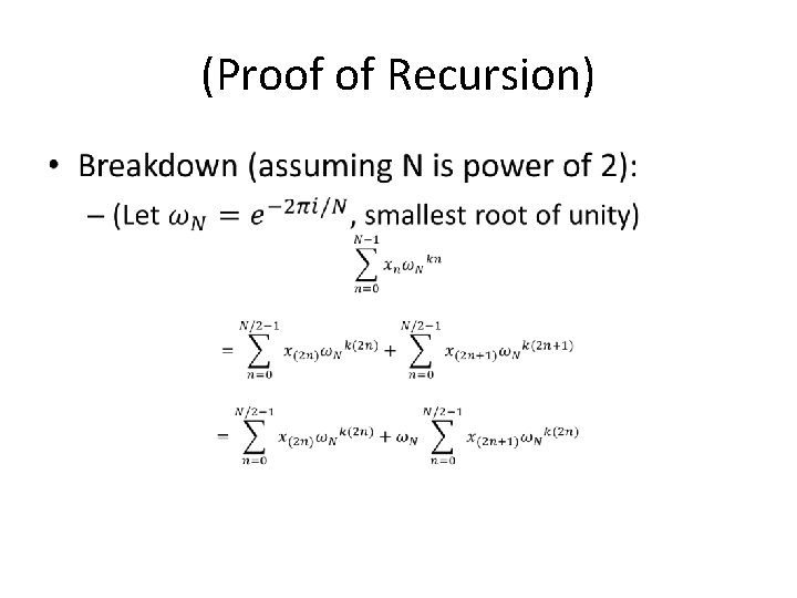
(Proof -- -- breaks DFT into two DFTs, even/odd) • kk kkkk

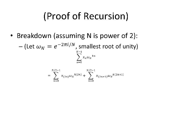
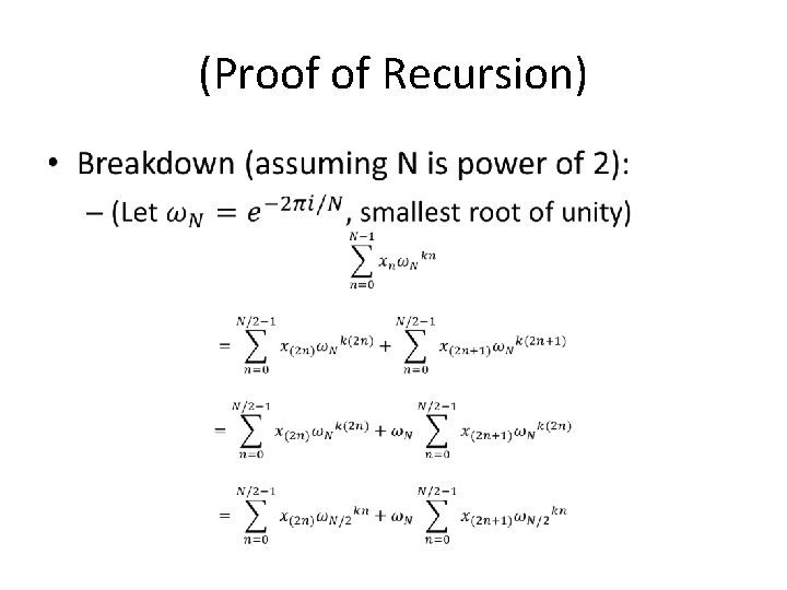
(Proof of Recursion) •

(Proof of Recursion) •

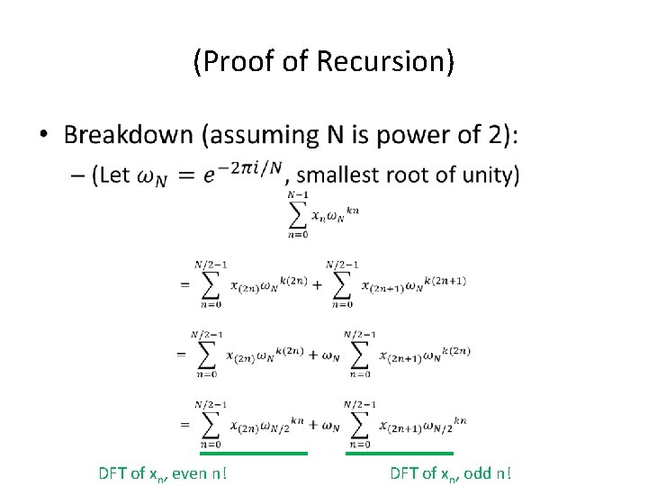
(Proof of Recursion) •

(Proof of Recursion) • DFT of xn, even n! DFT of xn, odd n!

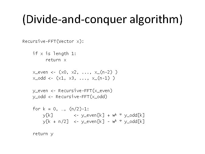
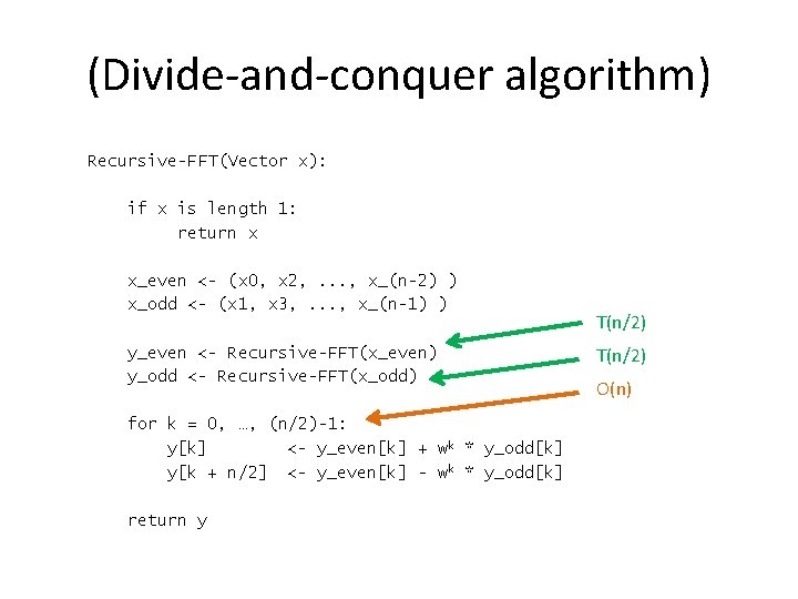
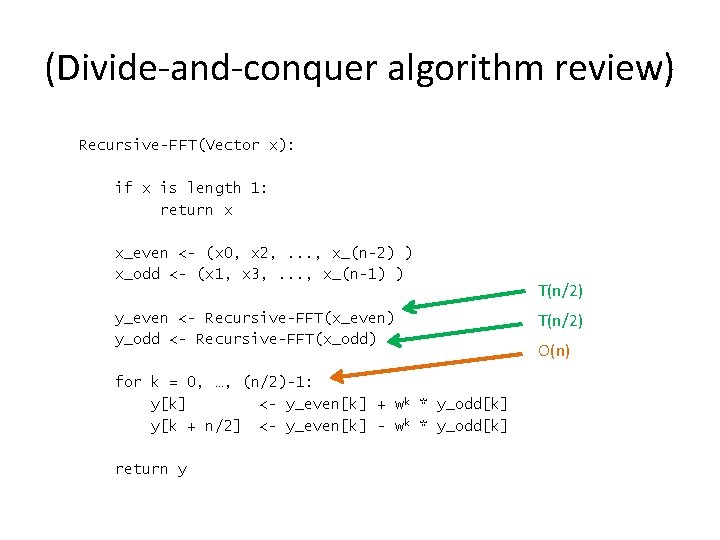
(Divide-and-conquer algorithm) Recursive-FFT(Vector x): if x is length 1: return x x_even <- (x 0, x 2, . . . , x_(n-2) ) x_odd <- (x 1, x 3, . . . , x_(n-1) ) y_even <- Recursive-FFT(x_even) y_odd <- Recursive-FFT(x_odd) for k = 0, …, (n/2)-1: y[k] <- y_even[k] + wk * y_odd[k] y[k + n/2] <- y_even[k] - wk * y_odd[k] return y

(Divide-and-conquer algorithm) Recursive-FFT(Vector x): if x is length 1: return x x_even <- (x 0, x 2, . . . , x_(n-2) ) x_odd <- (x 1, x 3, . . . , x_(n-1) ) y_even <- Recursive-FFT(x_even) y_odd <- Recursive-FFT(x_odd) for k = 0, …, (n/2)-1: y[k] <- y_even[k] + wk * y_odd[k] y[k + n/2] <- y_even[k] - wk * y_odd[k] return y T(n/2) O(n)

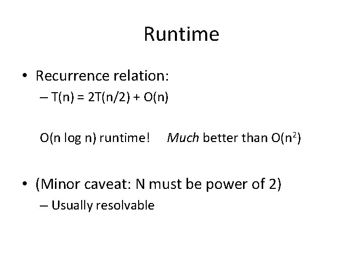
Runtime • Recurrence relation: – T(n) = 2 T(n/2) + O(n) O(n log n) runtime! Much better than O(n 2) • (Minor caveat: N must be power of 2) – Usually resolvable

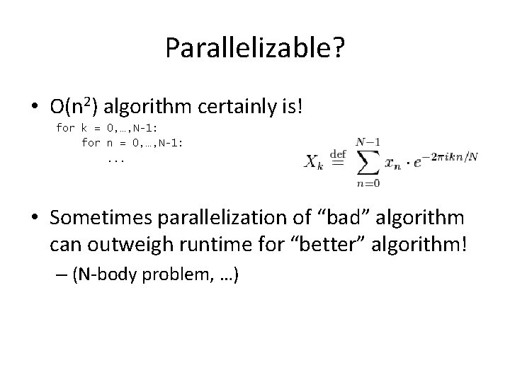
Parallelizable? • O(n 2) algorithm certainly is! for k = 0, …, N-1: for n = 0, …, N-1: . . . • Sometimes parallelization of “bad” algorithm can outweigh runtime for “better” algorithm! – (N-body problem, …)

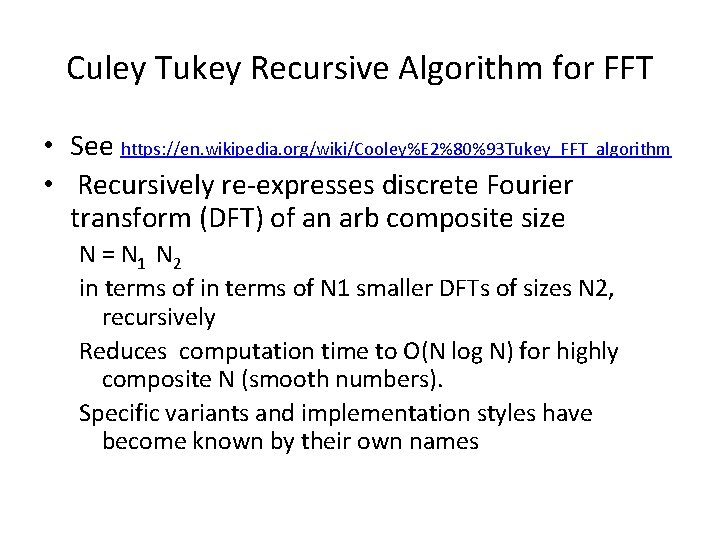
Culey Tukey Recursive Algorithm for FFT • See https: //en. wikipedia. org/wiki/Cooley%E 2%80%93 Tukey_FFT_algorithm • Recursively re-expresses discrete Fourier transform (DFT) of an arb composite size N = N 1 N 2 in terms of N 1 smaller DFTs of sizes N 2, recursively Reduces computation time to O(N log N) for highly composite N (smooth numbers). Specific variants and implementation styles have become known by their own names

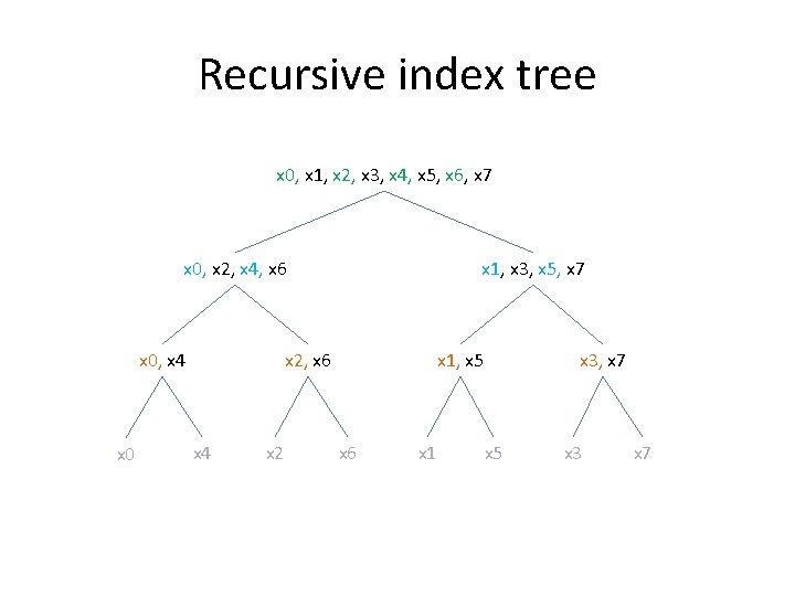
Recursive index tree x 0, x 1, x 2, x 3, x 4, x 5, x 6, x 7 x 0, x 2, x 4, x 6 x 0, x 4 x 0 x 1, x 3, x 5, x 7 x 2, x 6 x 4 x 2 x 1, x 5 x 6 x 1 x 3, x 7 x 5 x 3 x 7

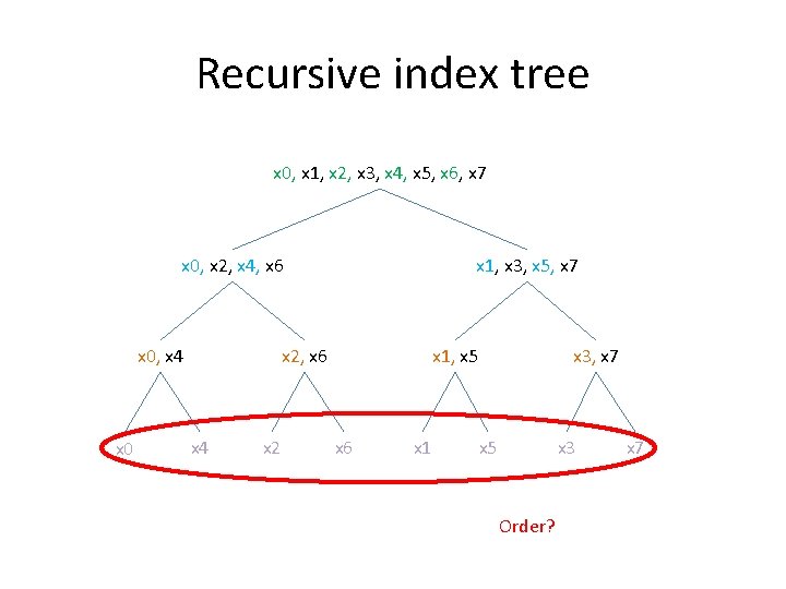
Recursive index tree x 0, x 1, x 2, x 3, x 4, x 5, x 6, x 7 x 0, x 2, x 4, x 6 x 0, x 4 x 0 x 1, x 3, x 5, x 7 x 2, x 6 x 4 x 2 x 1, x 5 x 6 x 1 x 3, x 7 x 5 x 3 Order? x 7

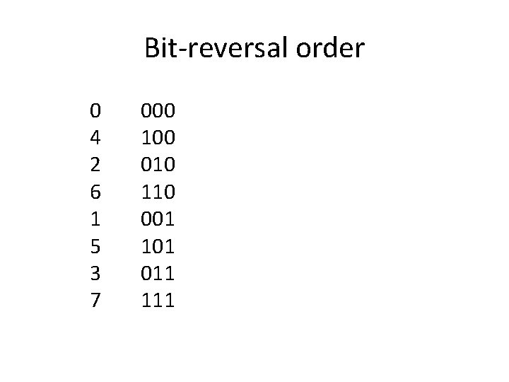
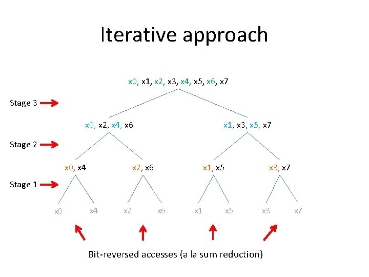
Bit-reversal order 0 4 2 6 1 5 3 7 000 100 010 110 001 101 011 111

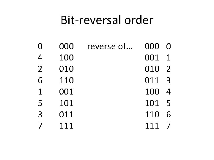
Bit-reversal order 0 4 2 6 1 5 3 7 000 100 010 110 001 101 011 111 reverse of… 000 001 010 011 100 101 110 111 0 1 2 3 4 5 6 7

(Divide-and-conquer algorithm review) Recursive-FFT(Vector x): if x is length 1: return x x_even <- (x 0, x 2, . . . , x_(n-2) ) x_odd <- (x 1, x 3, . . . , x_(n-1) ) y_even <- Recursive-FFT(x_even) y_odd <- Recursive-FFT(x_odd) for k = 0, …, (n/2)-1: y[k] <- y_even[k] + wk * y_odd[k] y[k + n/2] <- y_even[k] - wk * y_odd[k] return y T(n/2) O(n)

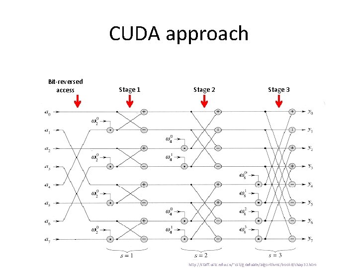
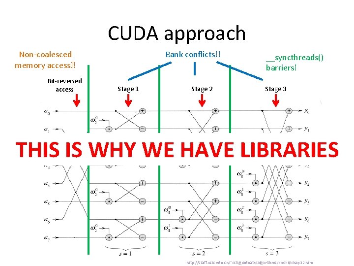
Iterative approach x 0, x 1, x 2, x 3, x 4, x 5, x 6, x 7 Stage 3 x 0, x 2, x 4, x 6 x 1, x 3, x 5, x 7 Stage 2 x 0, x 4 x 2, x 6 x 1, x 5 x 3, x 7 Stage 1 x 0 x 4 x 2 x 6 x 1 x 5 x 3 Bit-reversed accesses (a la sum reduction) x 7

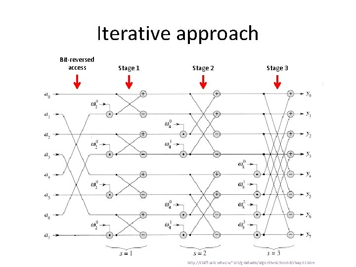
Iterative approach Bit-reversed access Stage 1 Stage 2 Stage 3 http: //staff. ustc. edu. cn/~csli/graduate/algorithms/book 6/chap 32. htm

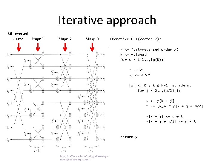
Iterative approach Bit-reversed access Stage 1 Stage 2 Stage 3 Iterative-FFT(Vector x): y <- (bit-reversed order x) N <- y. length for s = 1, 2, …, lg(N): m <- 2 s wn <- e 2πj/m for k: 0 ≤ k ≤ N-1, stride m: for j = 0, …, (m/2)-1: u <- y[k + j] t <- (w n)j * y[k + j + m/2] y[k + j] <- u + t y[k + j + m/2] <- u - t return y http: //staff. ustc. edu. cn/~csli/graduate/algo rithms/book 6/chap 32. htm

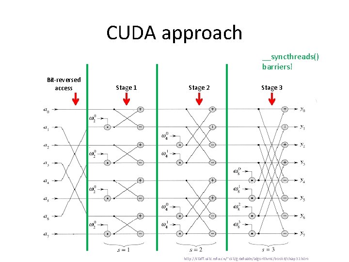
CUDA approach Bit-reversed access Stage 1 Stage 2 Stage 3 http: //staff. ustc. edu. cn/~csli/graduate/algorithms/book 6/chap 32. htm

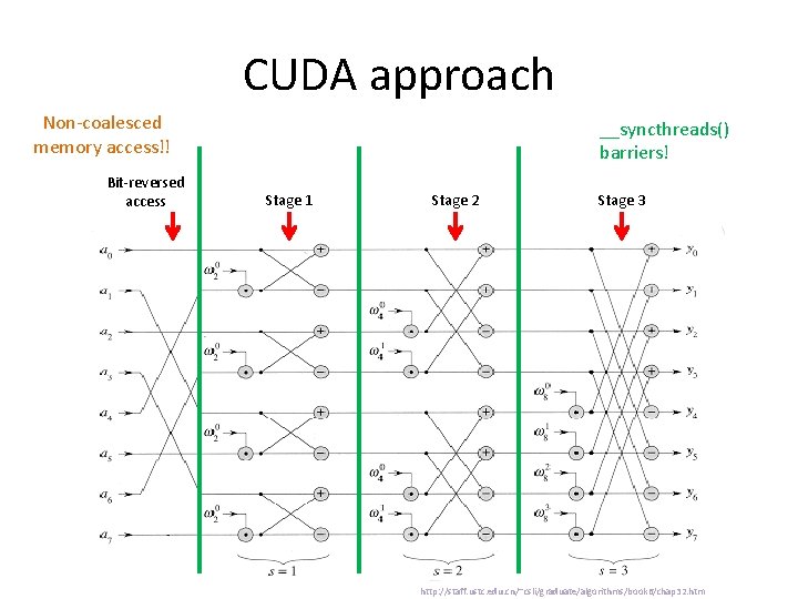
CUDA approach __syncthreads() barriers! Bit-reversed access Stage 1 Stage 2 Stage 3 http: //staff. ustc. edu. cn/~csli/graduate/algorithms/book 6/chap 32. htm

CUDA approach Non-coalesced memory access!! Bit-reversed access __syncthreads() barriers! Stage 1 Stage 2 Stage 3 http: //staff. ustc. edu. cn/~csli/graduate/algorithms/book 6/chap 32. htm

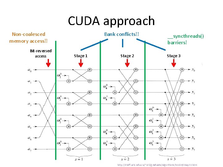
CUDA approach Non-coalesced memory access!! Bit-reversed access Bank conflicts!! Stage 1 Stage 2 __syncthreads() barriers! Stage 3 http: //staff. ustc. edu. cn/~csli/graduate/algorithms/book 6/chap 32. htm

CUDA approach Non-coalesced memory access!! Bit-reversed access Bank conflicts!! Stage 1 Stage 2 __syncthreads() barriers! Stage 3 THIS IS WHY WE HAVE LIBRARIES http: //staff. ustc. edu. cn/~csli/graduate/algorithms/book 6/chap 32. htm

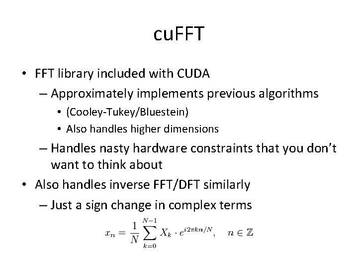
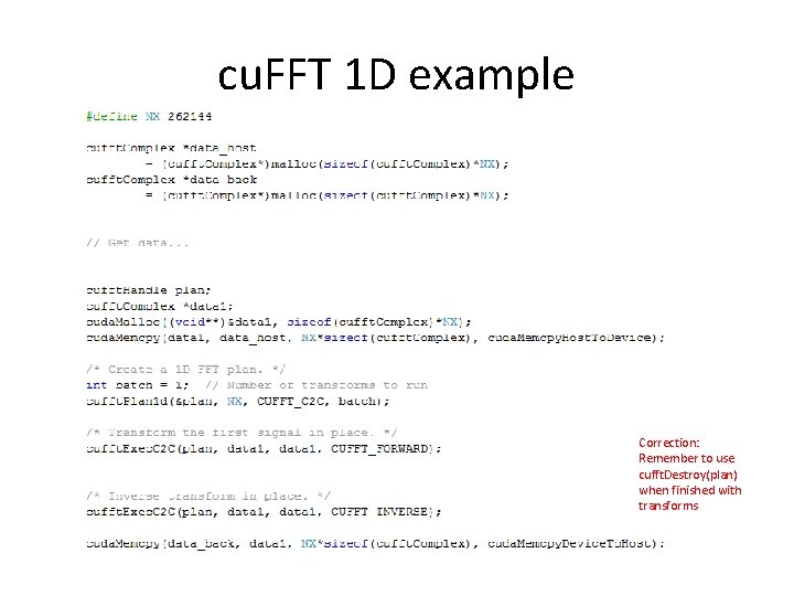
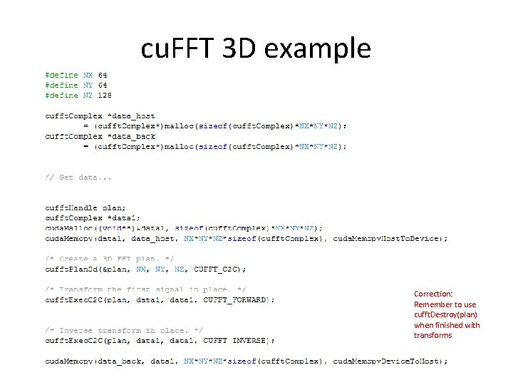
cu. FFT • FFT library included with CUDA – Approximately implements previous algorithms • (Cooley-Tukey/Bluestein) • Also handles higher dimensions – Handles nasty hardware constraints that you don’t want to think about • Also handles inverse FFT/DFT similarly – Just a sign change in complex terms

cu. FFT 1 D example Correction: Remember to use cufft. Destroy(plan) when finished with transforms

cu. FFT 3 D example Correction: Remember to use cufft. Destroy(plan) when finished with transforms

Remarks • As before, some parallelizable algorithms don’t easily “fit the mold” – Hardware matters more! • Some resources: – Introduction to Algorithms (Cormen, et al), aka “CLRS”, esp. Sec 30. 5 – “An Efficient Implementation of Double Precision 1 -D FFT for GPUs Using CUDA” (Liu, et al. )