Confidence intervals fundamental issues Null Hypothesis testing Pvalues

Confidence intervals fundamental issues —Null Hypothesis testing – P-values — Classical or ‘frequentist’ confidence intervals — Issues that arise in interpretation of fit result — Bayesian statistics and intervals Wouter Verkerke, UCSB

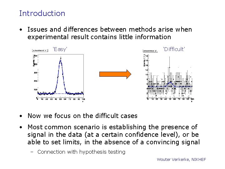
Introduction • Issues and differences between methods arise when experimental result contains little information ‘Easy’ ‘Difficult’ • Now we focus on the difficult cases • Most common scenario is establishing the presence of signal in the data (at a certain confidence level), or be able to set limits, in the absence of a convincing signal – Connection with hypothesis testing Wouter Verkerke, NIKHEF

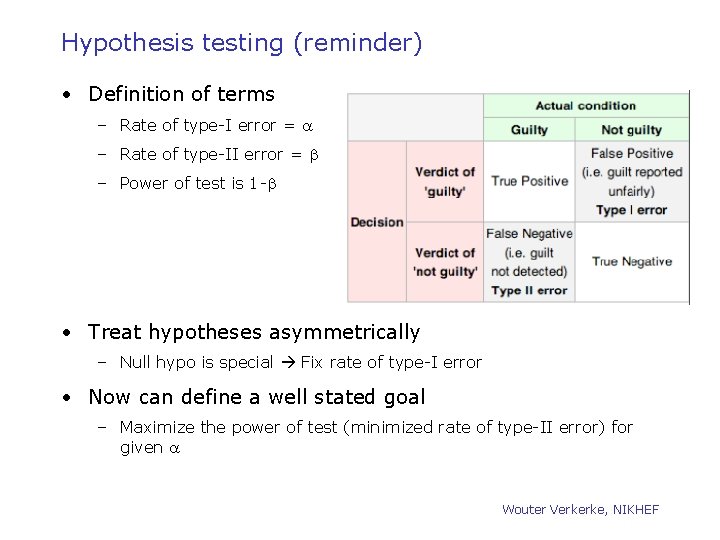
Hypothesis testing (reminder) • Definition of terms – Rate of type-I error = a – Rate of type-II error = b – Power of test is 1 -b • Treat hypotheses asymmetrically – Null hypo is special Fix rate of type-I error • Now can define a well stated goal – Maximize the power of test (minimized rate of type-II error) for given a Wouter Verkerke, NIKHEF

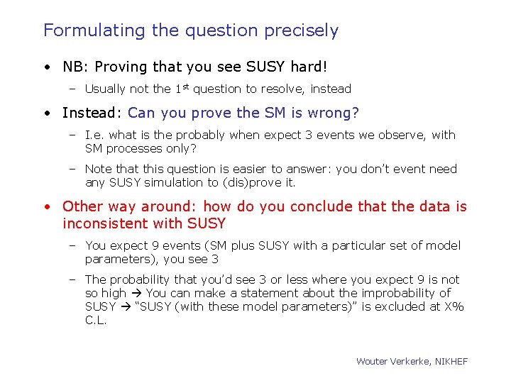
Formulating the question precisely • When making statistical inference on data samples that contain little information, precise formulation of question and assumption made, become very important • Let’s start with a very basic formulation on the question of discovery. • Hypothetical case for “Super. Symmetry” discovery – Simulation for SM – Predicts 3 events (Poisson, μ exactly known) – Simulation for SUSY – Predicts 6 events 9 events in total – Observed event count in data: 8 events • How do you conclude (or not) that you’ve discovered supersymmetry? – You expect 9 events (with SUSY), you see 8, looks promising Wouter Verkerke, NIKHEF

Formulating the question precisely • NB: Proving that you see SUSY hard! – Usually not the 1 st question to resolve, instead • Instead: Can you prove the SM is wrong? – I. e. what is the probably when expect 3 events we observe, with SM processes only? – Note that this question is easier to answer: you don’t event need any SUSY simulation to (dis)prove it. • Other way around: how do you conclude that the data is inconsistent with SUSY – You expect 9 events (SM plus SUSY with a particular set of model parameters), you see 3 – The probability that you’d see 3 or less where you expect 9 is not so high You can make a statement about the improbability of SUSY “SUSY (with these model parameters)” is excluded at X% C. L. Wouter Verkerke, NIKHEF

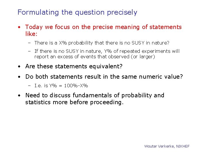
Formulating the question precisely • Today we focus on the precise meaning of statements like: – There is a X% probability that there is no SUSY in nature? – If there is no SUSY in nature, Y% of repeated experiments will report an excess of events that observed (or larger) • Are these statements equivalent? • Do both statements result in the same numeric value? – I. e. is Y% = 100%-X% • Need to discuss fundamentals of probability and statistics more before proceeding. Wouter Verkerke, NIKHEF

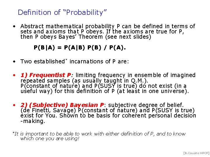
Definition of “Probability” • Abstract mathematical probability P can be defined in terms of sets and axioms that P obeys. If the axioms are true for P, then P obeys Bayes’ Theorem (see next slides) P(B|A) = P(A|B) P(B) / P(A). • Two established* incarnations of P are: • 1) Frequentist P: limiting frequency in ensemble of imagined repeated samples (as usually taught in Q. M. ). P(constant of nature) and P(SUSY is true) do not exist (in a useful way) for this definition of P (at least in one universe). • 2) (Subjective) Bayesian P: subjective degree of belief. (de Finetti, Savage) P(constant of nature) and P(SUSY is true) exist for You. Shown to be basis for coherent personal decision -making. *It is important to be able to work with either definition of P, and to know which one you are using! [B. Cousins HPCP]

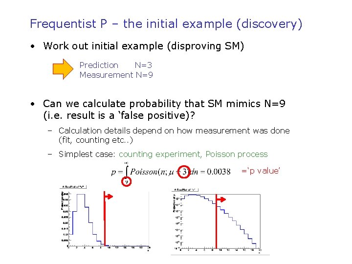
Frequentist P – the initial example (discovery) • Work out initial example (disproving SM) Prediction N=3 Measurement N=9 • Can we calculate probability that SM mimics N=9 (i. e. result is a ‘false positive)? – Calculation details depend on how measurement was done (fit, counting etc. . ) – Simplest case: counting experiment, Poisson process =‘p value’

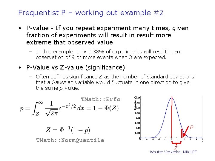
Frequentist P – working out example #2 • P-value - If you repeat experiment many times, given fraction of experiments will result in result more extreme that observed value – In this example, only 0. 38% of experiments will result in an observation of 9 or more events when 3 are expected. • P-Value vs Z-value (significance) – Often defines significance Z as the number of standard deviations that a Gaussian variable would fluctuate in one direction to give the same p-value. TMath: : Erfc p TMath: : Norm. Quantile Z Wouter Verkerke, NIKHEF

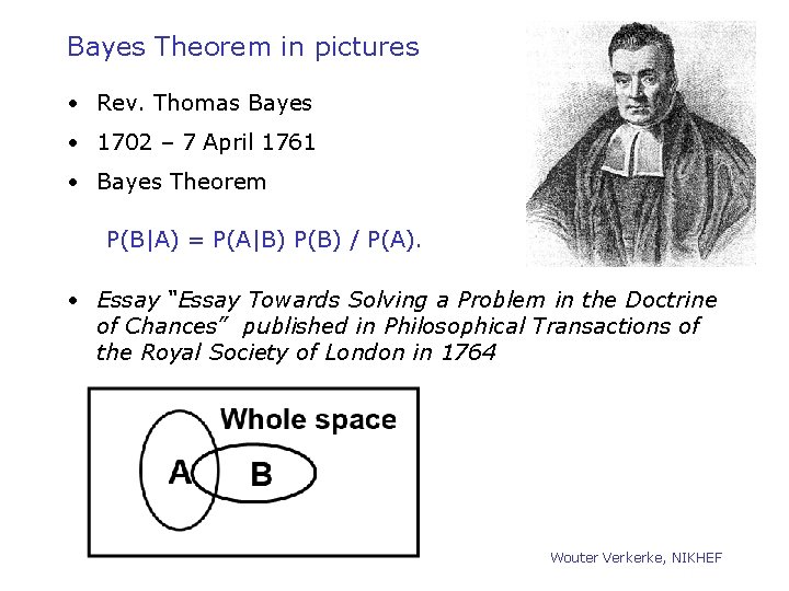
Bayes Theorem in pictures • Rev. Thomas Bayes • 1702 – 7 April 1761 • Bayes Theorem P(B|A) = P(A|B) P(B) / P(A). • Essay “Essay Towards Solving a Problem in the Doctrine of Chances” published in Philosophical Transactions of the Royal Society of London in 1764 Wouter Verkerke, NIKHEF

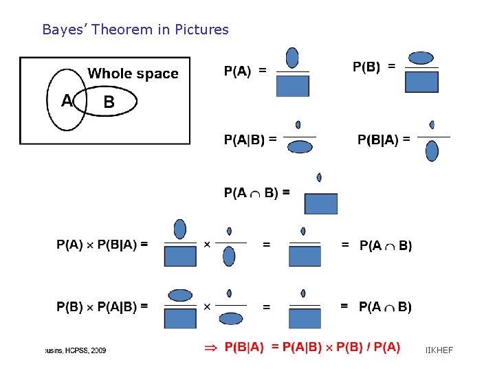
Bayes’ Theorem in Pictures Wouter Verkerke, NIKHEF

What is the “Whole Space”? • Note that for probabilities to be well-defined, the “whole space” needs to be defined, which in practice introduces assumptions and restrictions. • Thus the “whole space” itself is more properly thought of as a conditional space, conditional on the assumptions going into the model (Poisson process, whether or not total number of events was fixed, etc. ). • Furthermore, it is widely accepted that restricting the “whole space” to a relevant subspace can sometimes improve the quality of statistical inference –see the discussion of “Conditioning” in later slides. Wouter Verkerke, NIKHEF [B. Cousins HPCP]

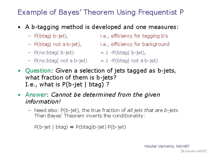
Example of Bayes’ Theorem Using Frequentist P • A b-tagging method is developed and one measures: – P(btag| b-jet), i. e. , efficiency for tagging b’s – P(btag| not a b-jet), i. e. , efficiency for background – P(no btag| b-jet) = 1 -P(btag| b-jet), – P(no btag| not a b-jet) = 1 -P(btag| not a b-jet) • Question: Given a selection of jets tagged as b-jets, what fraction of them is b-jets? I. e. , what is P(b-jet | btag) ? • Answer: Cannot be determined from the given information! – Need also: P(b-jet), the true fraction of all jets that are b-jets. Then Bayes’ Theorem inverts the conditionality: P(b-jet | btag) ∝ P(btag|b-jet) P(b-jet) Wouter Verkerke, NIKHEF [B. Cousins HPCP]

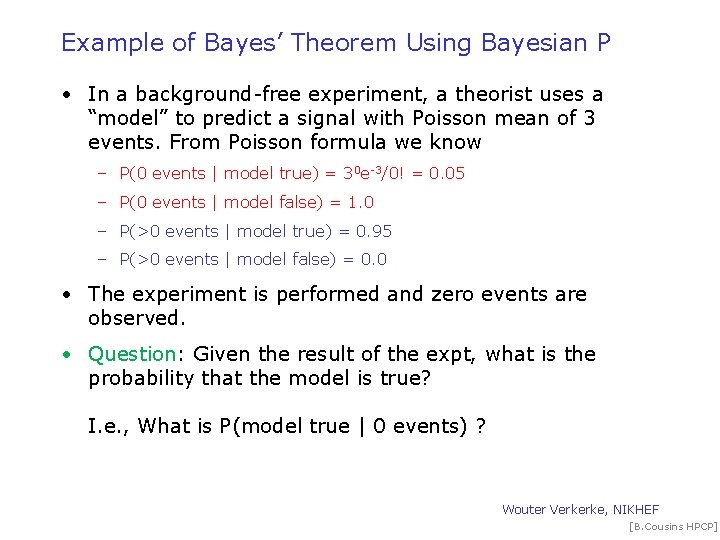
Example of Bayes’ Theorem Using Bayesian P • In a background-free experiment, a theorist uses a “model” to predict a signal with Poisson mean of 3 events. From Poisson formula we know – P(0 events | model true) = 30 e-3/0! = 0. 05 – P(0 events | model false) = 1. 0 – P(>0 events | model true) = 0. 95 – P(>0 events | model false) = 0. 0 • The experiment is performed and zero events are observed. • Question: Given the result of the expt, what is the probability that the model is true? I. e. , What is P(model true | 0 events) ? Wouter Verkerke, NIKHEF [B. Cousins HPCP]

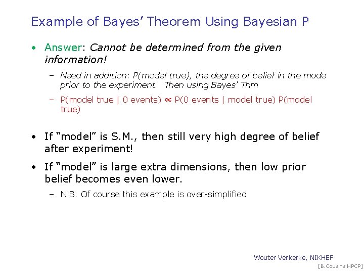
Example of Bayes’ Theorem Using Bayesian P • Answer: Cannot be determined from the given information! – Need in addition: P(model true), the degree of belief in the mode prior to the experiment. Then using Bayes’ Thm – P(model true | 0 events) ∝ P(0 events | model true) P(model true) • If “model” is S. M. , then still very high degree of belief after experiment! • If “model” is large extra dimensions, then low prior belief becomes even lower. – N. B. Of course this example is over-simplified Wouter Verkerke, NIKHEF [B. Cousins HPCP]

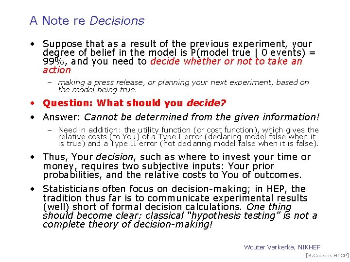
A Note re Decisions • Suppose that as a result of the previous experiment, your degree of belief in the model is P(model true | 0 events) = 99%, and you need to decide whether or not to take an action – making a press release, or planning your next experiment, based on the model being true. • Question: What should you decide? • Answer: Cannot be determined from the given information! – Need in addition: the utility function (or cost function), which gives the relative costs (to You) of a Type I error (declaring model false when it is true) and a Type II error (not declaring model false when it is false). • Thus, Your decision, such as where to invest your time or money, requires two subjective inputs: Your prior probabilities, and the relative costs to You of outcomes. • Statisticians often focus on decision-making; in HEP, the tradition thus far is to communicate experimental results (well) short of formal decision calculations. One thing should become clear: classical “hypothesis testing” is not a complete theory of decision-making! Wouter Verkerke, NIKHEF [B. Cousins HPCP]

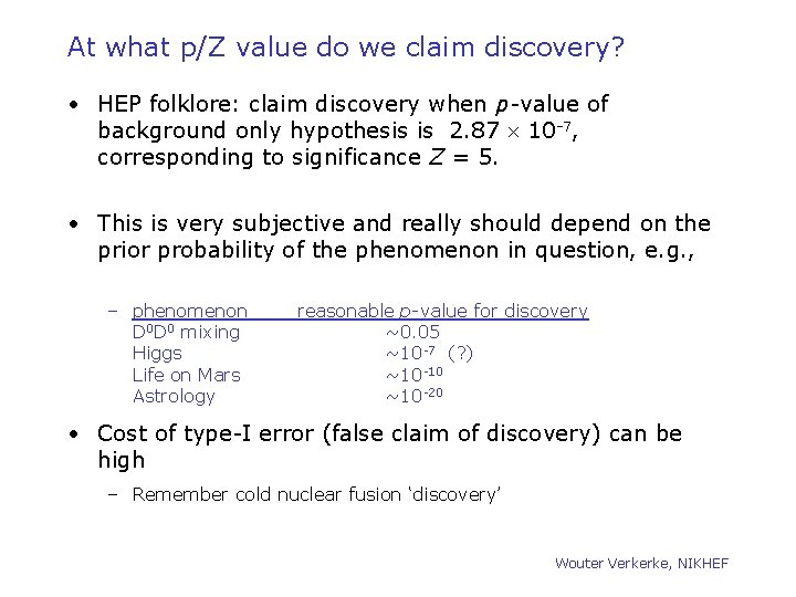
At what p/Z value do we claim discovery? • HEP folklore: claim discovery when p-value of background only hypothesis is 2. 87 10 -7, corresponding to significance Z = 5. • This is very subjective and really should depend on the prior probability of the phenomenon in question, e. g. , – phenomenon D 0 D 0 mixing Higgs Life on Mars Astrology reasonable p-value for discovery ~0. 05 ~10 -7 (? ) ~10 -10 ~10 -20 • Cost of type-I error (false claim of discovery) can be high – Remember cold nuclear fusion ‘discovery’ Wouter Verkerke, NIKHEF

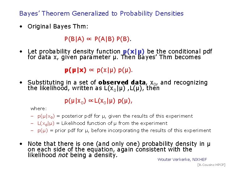
Bayes’ Theorem Generalized to Probability Densities • Original Bayes Thm: P(B|A) ∝ P(A|B) P(B). • Let probability density function p(x|μ) be the conditional pdf for data x, given parameter μ. Then Bayes’ Thm becomes p(μ|x) ∝ p(x|μ) p(μ). • Substituting in a set of observed data, x 0, and recognizing the likelihood, written as L(x 0|μ) , L(μ), then p(μ|x 0) ∝L(x 0|μ) p(μ), where: – p(μ|x 0) = posterior pdf for μ, given the results of this experiment – L(x 0|μ) = Likelihood function of μ from the experiment – p(μ) = prior pdf for μ, before incorporating the results of this experiment • Note that there is one (and only one) probability density in μ on each side of the equation, again consistent with the likelihood not being a density. Wouter Verkerke, NIKHEF [B. Cousins HPCP]

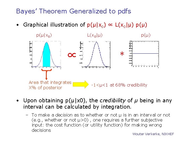
Bayes’ Theorem Generalized to pdfs • Graphical illustration of p(μ|x 0) ∝ L(x 0|μ) p(μ|x 0) L(x 0|μ) ∝ Area that integrates X% of posterior p(μ) ∗ -1<μ<1 at 68% credibility • Upon obtaining p(μ|x 0), the credibility of μ being in any interval can be calculated by integration. – To make a decision as to whether or not μ is in an interval or not (e. g. , whether or not μ>0) , one requires a further subjective input: the cost function (or utility function) for making wrong decisions Wouter Verkerke, NIKHEF

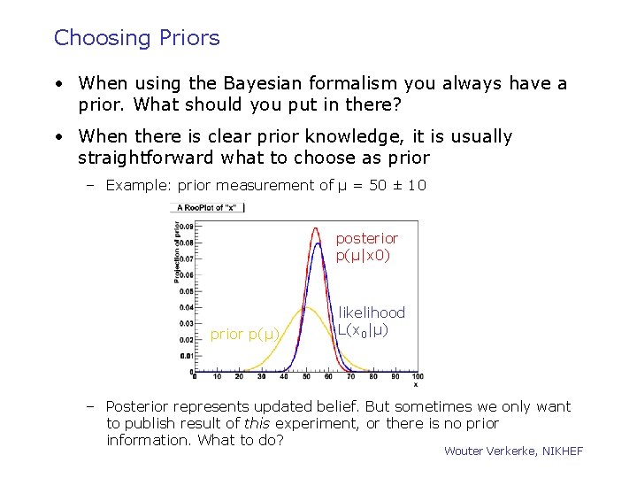
Choosing Priors • When using the Bayesian formalism you always have a prior. What should you put in there? • When there is clear prior knowledge, it is usually straightforward what to choose as prior – Example: prior measurement of μ = 50 ± 10 posterior p(μ|x 0) prior p(μ) likelihood L(x 0|μ) – Posterior represents updated belief. But sometimes we only want to publish result of this experiment, or there is no prior information. What to do? Wouter Verkerke, NIKHEF

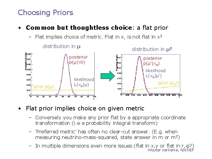
Choosing Priors • Common but thoughtless choice: a flat prior – Flat implies choice of metric. Flat in x, is not flat in x 2 distribution in μ posterior p(μ|x 0) prior p(μ) distribution in μ 2 posterior p(μ’|x 0) likelihood L(x 0|μ’) prior p(μ’) • Flat prior implies choice on given metric – Conversely you make any prior flat by a appropriate coordinate transformation (i. e a probability integral transform) – ‘Preferred metric’ has often no clear-cut answer. (E. g. when measuring neutrino-mass-squared, state answer in m or m 2) – In multiple dimensions even more issues (flat in x, y or flat in r, φ? ) Wouter Verkerke, NIKHEF

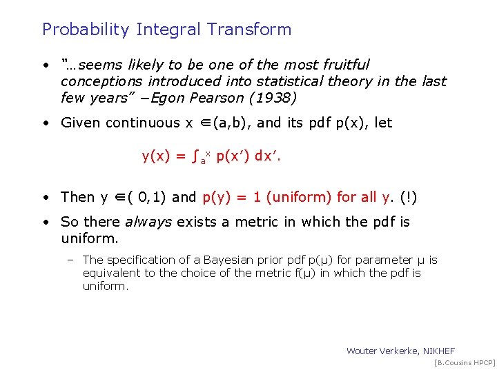
Probability Integral Transform • “…seems likely to be one of the most fruitful conceptions introduced into statistical theory in the last few years” −Egon Pearson (1938) • Given continuous x ∈(a, b), and its pdf p(x), let y(x) = ∫ax p(x′) dx′. • Then y ∈( 0, 1) and p(y) = 1 (uniform) for all y. (!) • So there always exists a metric in which the pdf is uniform. – The specification of a Bayesian prior pdf p(μ) for parameter μ is equivalent to the choice of the metric f(μ) in which the pdf is uniform. Wouter Verkerke, NIKHEF [B. Cousins HPCP]

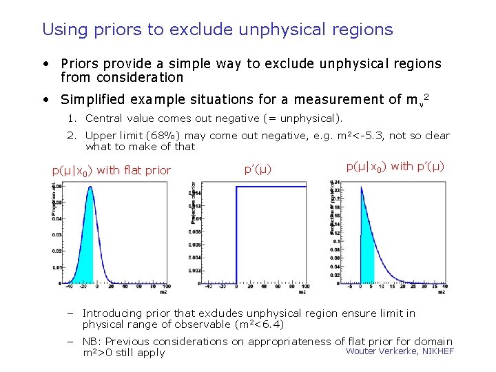
Using priors to exclude unphysical regions • Priors provide a simple way to exclude unphysical regions from consideration • Simplified example situations for a measurement of mn 2 1. Central value comes out negative (= unphysical). 2. Upper limit (68%) may come out negative, e. g. m 2<-5. 3, not so clear what to make of that p(μ|x 0) with flat prior p’(μ) p(μ|x 0) with p’(μ) – Introducing prior that excludes unphysical region ensure limit in physical range of observable (m 2<6. 4) – NB: Previous considerations on appropriateness of flat prior for domain Wouter Verkerke, NIKHEF m 2>0 still apply

Non-subjective priors? • The question is: can the Bayesian formalism be used by scientists to report the results of their experiments in an “objective” way (however one defines “objective”), and does any of the coherence remain when subjective P is replaced by something else? • Can one define a prior p(μ) which contains as little information as possible, so that the posterior pdf is dominated by the likelihood? – – • Unbounded mean μ of gaussian: p(μ) = 1 Poisson signal mean μ, no background: p(μ) = 1/sqrt(μ) Many ideas and names around on non-subjective priors – – • The really thoughtless idea*, recognized by Jeffreys as such, but dismayingly common in HEP: just choose p(μ) uniform in whatever metric you happen to be using! “Jeffreys Prior” answers the question using a prior uniform in a metric related to the Fisher information. – – • A bright idea, vigorously pursued by physicist Harold Jeffreys in in mid-20 thcentury: Objective priors? Non-informative priors? Uninformative priors? Vague priors? Ignorance priors? Reference priors? Kassand & Wasserman who have compiled a list of them, suggest a neutral name : Priors selected by “formal rules”. – Whatever the name, keep in mind that choice of prior in one metric determines it in all other metrics: be careful in the choice of metric in which it is uniform! – N. B. When professional statisticians refer to “flat prior”, they usually mean the Jeffreys prior. Wouter Verkerke, NIKHEF [B. Cousins HPCP]

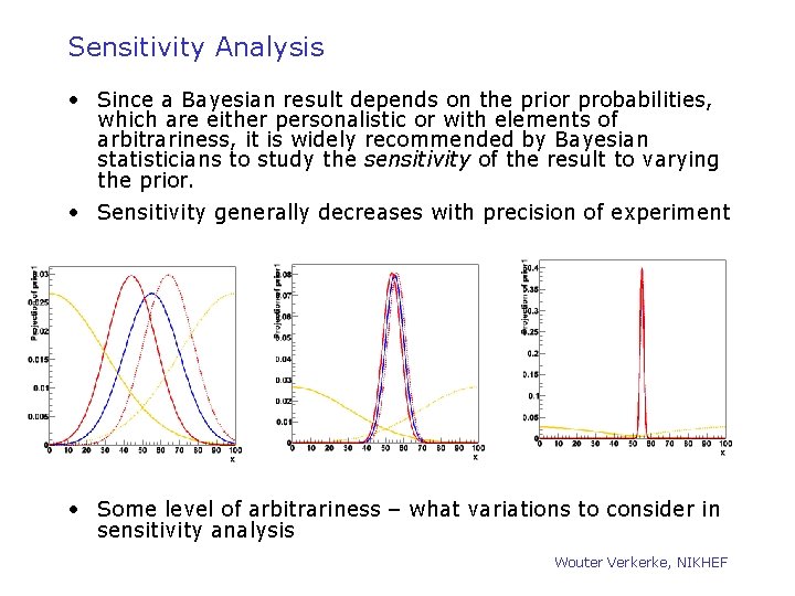
Sensitivity Analysis • Since a Bayesian result depends on the prior probabilities, which are either personalistic or with elements of arbitrariness, it is widely recommended by Bayesian statisticians to study the sensitivity of the result to varying the prior. • Sensitivity generally decreases with precision of experiment • Some level of arbitrariness – what variations to consider in sensitivity analysis Wouter Verkerke, NIKHEF

Bayesian Probability • Bayesian probability is often the ‘natural’ framework in which people (& scientists) think. • If you read “ 90 < M(X) < 100” to mean that the true M(X) has a 68% probability of being between 90 -100 then you’re thinking in terms of Bayesian probability • Strictly speaking your quantifying your belief in M(X) (or perhaps our ‘collective belief as HEP scientists’ as true value in nature of M(X) is fixed (but unknown) • In the Bayesian framework you always have a prior. – If you didn’t put one in, you’re assuming it to be flat in your current choice of metric Wouter Verkerke, NIKHEF

What Can Be Computed without Using a Prior? • Not P(constant of nature | data). 1. Confidence Intervals for parameter values, as defined in the 1930’s by Jerzy Neyman. 2. Likelihood ratios, the basis for a large set of techniques for point estimation, interval estimation, and hypothesis testing. • These can both be constructed using frequentist definition of P. • Compare and contrast them with Bayesian methods. Wouter Verkerke, NIKHEF [B. Cousins HPCP]

Confidence Intervals • “Confidence intervals”, and this phrase to describe them, were invented by Jerzy Neyman in 1934 -37. – While statisticians mean Neyman’s intervals (or an approximation) when they say “confidence interval”, in HEP the language tends to be a little loose. – Recommend using “confidence interval” only to describe intervals corresponding to Neyman’s construction (or good approximations thereof), described below. • The slides contain the crucial information, but you will want to cycle through them a few times to “take home” how the construction works, since it is really ingenious – perhaps a bit too ingenious given how often confidence intervals are misinterpreted. • In particular, you will understand that the confidence level does not tell you “how confident you are that the unknown true value is in the interval” –only a subjective Bayesian credible interval has that property! Wouter Verkerke, NIKHEF [B. Cousins HPCP]

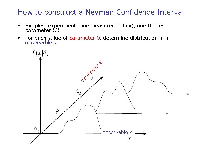
How to construct a Neyman Confidence Interval • Simplest experiment: one measurement (x), one theory parameter (q) • For each value of parameter θ, determine distribution in in observable x r te θ e pa am r observable x Wouter Verkerke, NIKHEF

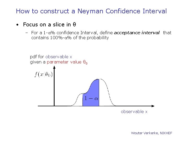
How to construct a Neyman Confidence Interval • Focus on a slice in θ – For a 1 -a% confidence Interval, define acceptance interval that contains 100%-a% of the probability pdf for observable x given a parameter value θ 0 observable x Wouter Verkerke, NIKHEF

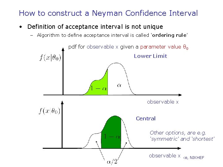
How to construct a Neyman Confidence Interval • Definition of acceptance interval is not unique – Algorithm to define acceptance interval is called ‘ordering rule’ pdf for observable x given a parameter value θ 0 Lower Limit observable x Central observable x Other options, are e. g. ‘symmetric’ and ‘shortest’ observable x Wouter Verkerke, NIKHEF

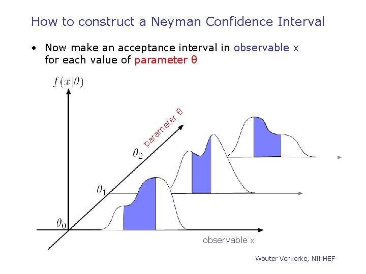
How to construct a Neyman Confidence Interval • Now make an acceptance interval in observable x for each value of parameter θ et er θ am r a p observable x Wouter Verkerke, NIKHEF

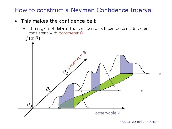
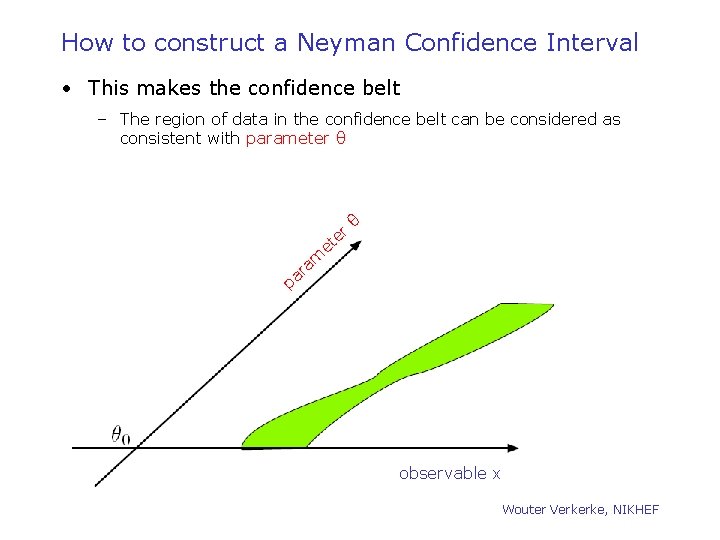
How to construct a Neyman Confidence Interval • This makes the confidence belt – The region of data in the confidence belt can be considered as consistent with parameter θ et er θ am r a p observable x Wouter Verkerke, NIKHEF

How to construct a Neyman Confidence Interval • This makes the confidence belt – The region of data in the confidence belt can be considered as consistent with parameter θ et er θ am r a p observable x Wouter Verkerke, NIKHEF

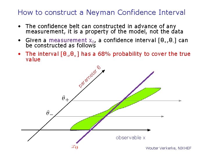
How to construct a Neyman Confidence Interval • The confidence belt can constructed in advance of any measurement, it is a property of the model, not the data • Given a measurement x 0, a confidence interval [θ+, θ-] can be constructed as follows • The interval [θ-, θ+] has a 68% probability to cover the true value r te θ e pa am r observable x Wouter Verkerke, NIKHEF

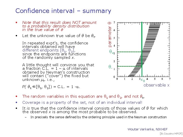
• Note that this result does NOT amount to a probability density distribution in the true value of q • Let the unknown true value of θ be θt. In repeated expt’s, the confidence intervals obtained will have different endpoints [θ 1, θ 2], since the endpoints are functions of the randomly sampled x. A little thought will convince you that a fraction C. L. = 1 – a of intervals obtained by Neyman’s construction will contain (“cover”) the fixed but unknown μt. i. e. , P( θt ∈[θ 1, θ 2]) = C. L. = 1 -a. parameter θ Confidence interval – summary θ+ θx 0 observable x • The random variables in this equation are θ 1 and θ 2, and not θt, • Coverage is a property of the set, not of an individual interval! • It is true that the confidence interval consists of those values of θ for which the observed x is among the most probable to be observed. – In precisely the sense defined by the ordering principle used in the Neyman construction Wouter Verkerke, NIKHEF [B. Cousins HPCP]

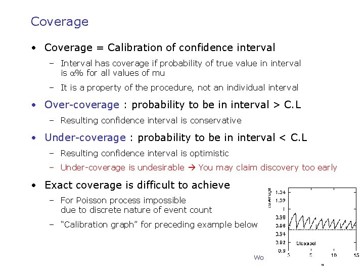
Coverage • Coverage = Calibration of confidence interval – Interval has coverage if probability of true value in interval is a% for all values of mu – It is a property of the procedure, not an individual interval • Over-coverage : probability to be in interval > C. L – Resulting confidence interval is conservative • Under-coverage : probability to be in interval < C. L – Resulting confidence interval is optimistic – Under-coverage is undesirable You may claim discovery too early • Exact coverage is difficult to achieve – For Poisson process impossible due to discrete nature of event count – “Calibration graph” for preceding example below Wouter Verkerke, NIKHEF

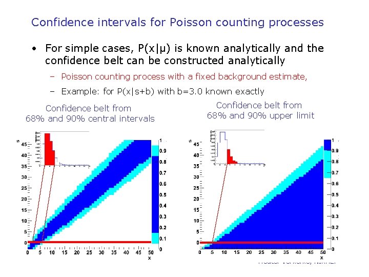
Confidence intervals for Poisson counting processes • For simple cases, P(x|μ) is known analytically and the confidence belt can be constructed analytically – Poisson counting process with a fixed background estimate, – Example: for P(x|s+b) with b=3. 0 known exactly Confidence belt from 68% and 90% central intervals Confidence belt from 68% and 90% upper limit Wouter Verkerke, NIKHEF

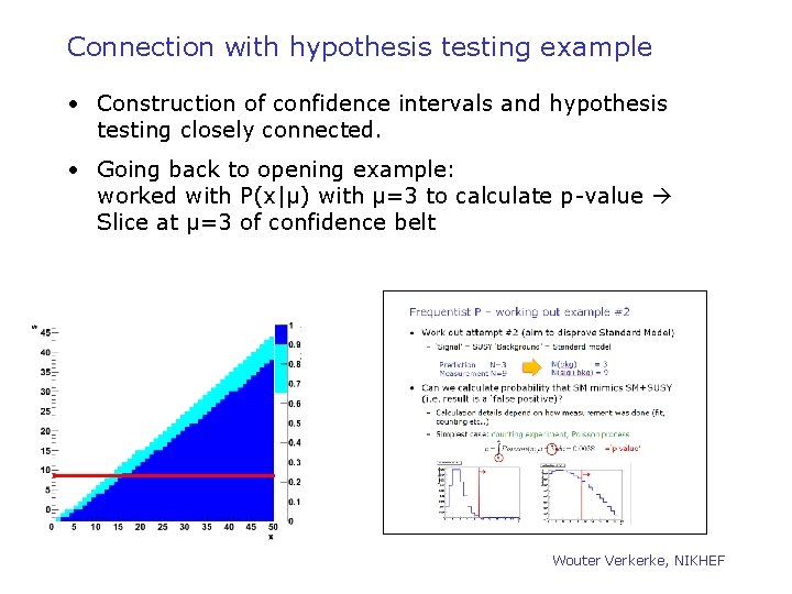
Connection with hypothesis testing example • Construction of confidence intervals and hypothesis testing closely connected. • Going back to opening example: worked with P(x|μ) with μ=3 to calculate p-value Slice at μ=3 of confidence belt Wouter Verkerke, NIKHEF

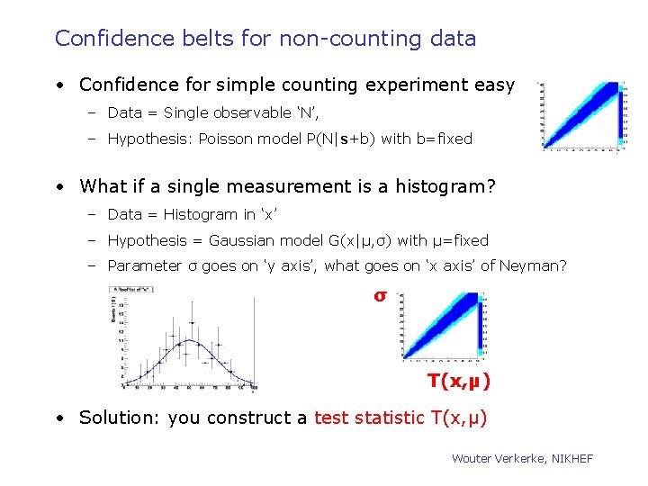
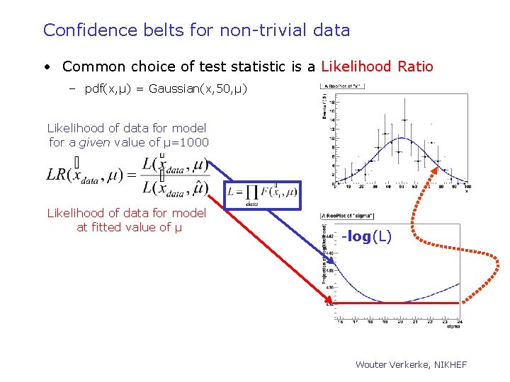
Confidence belts for non-counting data • Confidence for simple counting experiment easy – Data = Single observable ‘N’, – Hypothesis: Poisson model P(N|s+b) with b=fixed • What if a single measurement is a histogram? – Data = Histogram in ‘x’ – Hypothesis = Gaussian model G(x|μ, σ) with μ=fixed – Parameter σ goes on ‘y axis’, what goes on ‘x axis’ of Neyman? σ T(x, μ) • Solution: you construct a test statistic T(x, μ) Wouter Verkerke, NIKHEF

Confidence belts for non-trivial data • Common choice of test statistic is a Likelihood Ratio – pdf(x, μ) = Gaussian(x, 50, μ) Likelihood of data for model for a given value of μ=1000 Likelihood of data for model at fitted value of μ -log(L) Wouter Verkerke, NIKHEF

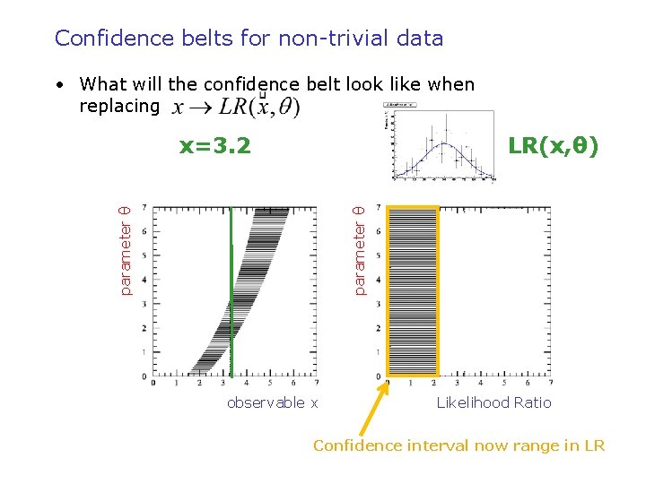
Confidence belts for non-trivial data • What will the confidence belt look like when replacing x=3. 2 parameter θ LR(x, θ) observable x Likelihood Ratio Confidence interval now range in LR

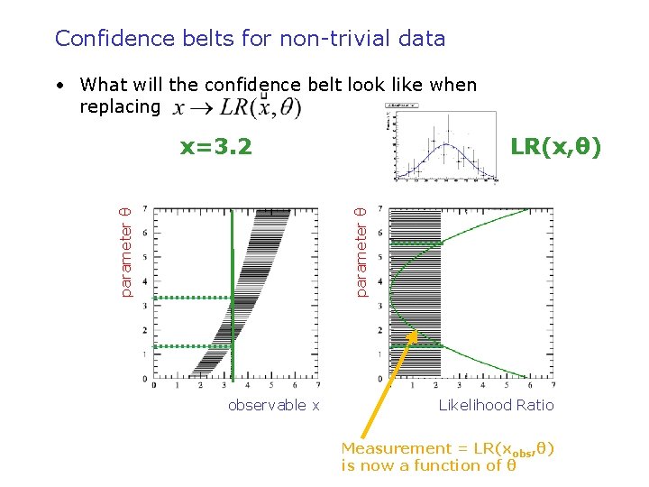
Confidence belts for non-trivial data • What will the confidence belt look like when replacing x=3. 2 parameter θ LR(x, θ) observable x Likelihood Ratio Measurement = LR(xobs, θ) is now a function of θ

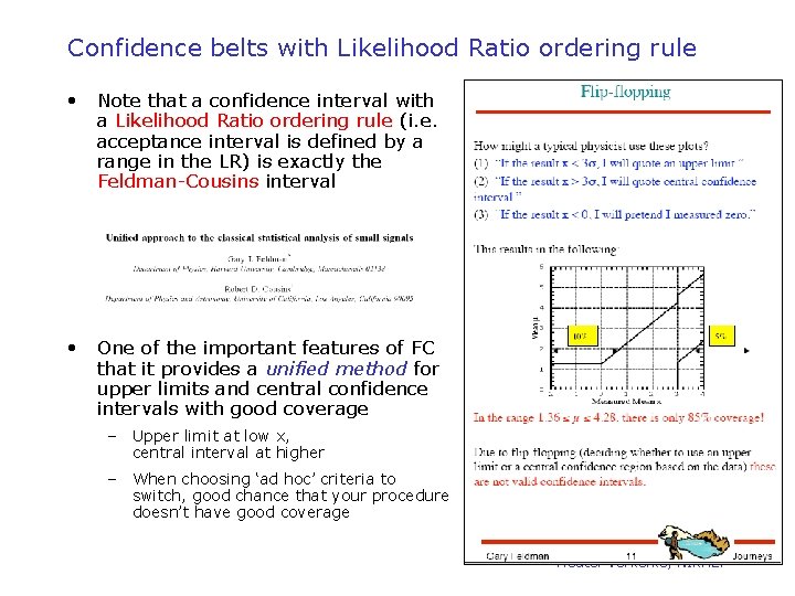
Confidence belts with Likelihood Ratio ordering rule • Note that a confidence interval with a Likelihood Ratio ordering rule (i. e. acceptance interval is defined by a range in the LR) is exactly the Feldman-Cousins interval • One of the important features of FC that it provides a unified method for upper limits and central confidence intervals with good coverage – Upper limit at low x, central interval at higher – When choosing ‘ad hoc’ criteria to switch, good chance that your procedure doesn’t have good coverage Wouter Verkerke, NIKHEF

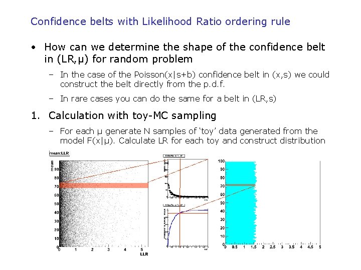
Confidence belts with Likelihood Ratio ordering rule • How can we determine the shape of the confidence belt in (LR, μ) for random problem – In the case of the Poisson(x|s+b) confidence belt in (x, s) we could construct the belt directly from the p. d. f. – In rare cases you can do the same for a belt in (LR, s) 1. Calculation with toy-MC sampling – For each μ generate N samples of ‘toy’ data generated from the model F(x|μ). Calculate LR for each toy and construct distribution

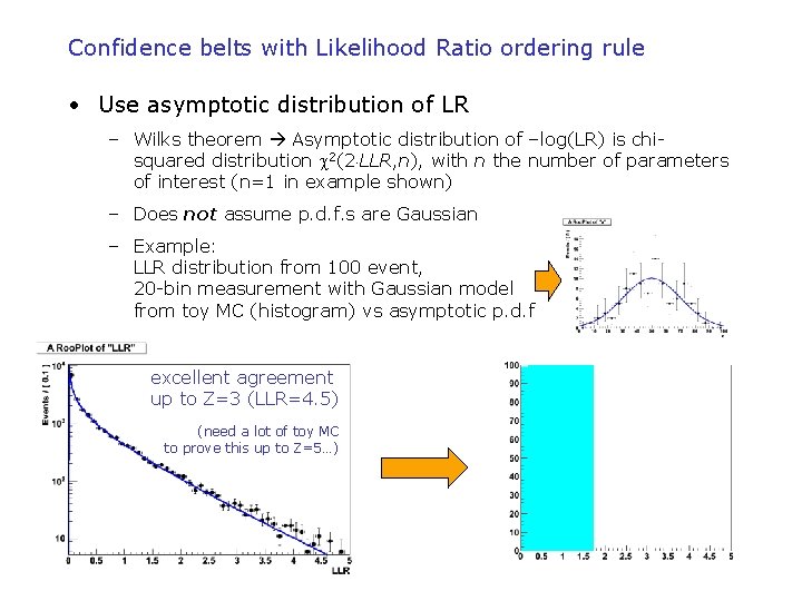
Confidence belts with Likelihood Ratio ordering rule • Use asymptotic distribution of LR – Wilks theorem Asymptotic distribution of –log(LR) is chisquared distribution 2(2 LLR, n), with n the number of parameters of interest (n=1 in example shown) – Does not assume p. d. f. s are Gaussian – Example: LLR distribution from 100 event, 20 -bin measurement with Gaussian model from toy MC (histogram) vs asymptotic p. d. f excellent agreement up to Z=3 (LLR=4. 5) (need a lot of toy MC to prove this up to Z=5…) Wouter Verkerke, NIKHEF

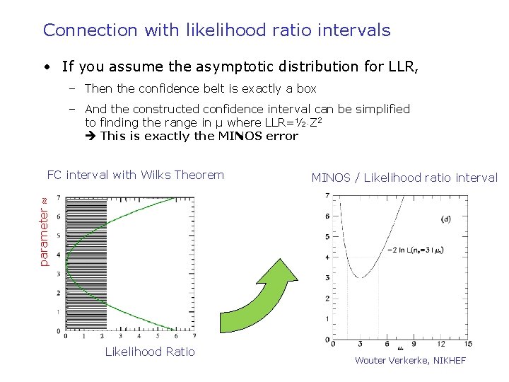
Connection with likelihood ratio intervals • If you assume the asymptotic distribution for LLR, – Then the confidence belt is exactly a box – And the constructed confidence interval can be simplified to finding the range in μ where LLR=½ Z 2 This is exactly the MINOS error MINOS / Likelihood ratio interval parameter FC interval with Wilks Theorem Likelihood Ratio Wouter Verkerke, NIKHEF

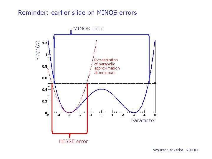
Reminder: earlier slide on MINOS errors -log. L(p) MINOS error Extrapolation of parabolic approximation at minimum Parameter HESSE error Wouter Verkerke, NIKHEF

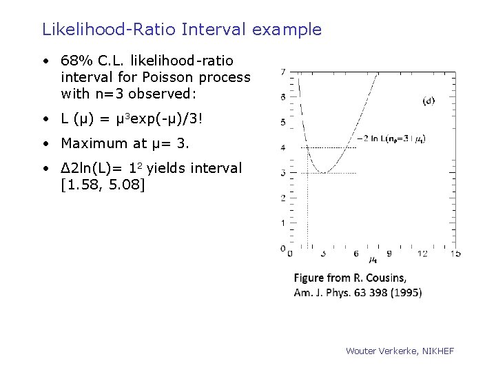
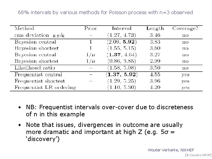
Likelihood-Ratio Interval example • 68% C. L. likelihood-ratio interval for Poisson process with n=3 observed: • L (μ) = μ 3 exp(-μ)/3! • Maximum at μ= 3. • Δ 2 ln(L)= 12 yields interval [1. 58, 5. 08] Wouter Verkerke, NIKHEF

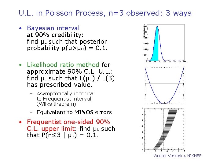
U. L. in Poisson Process, n=3 observed: 3 ways • Bayesian interval at 90% credibility: find μu such that posterior probability p(μ>μu) = 0. 1. • Likelihood ratio method for approximate 90% C. L. U. L. : find μu such that L(μu) / L(3) has prescribed value. – Asymptotically identical to Frequentist interval (Wilks theorem) – Equivalent to MINOS errors • Frequentist one-sided 90% C. L. upper limit: find μu such that P(n≤ 3 | μu) = 0. 1. Wouter Verkerke, NIKHEF

U. L. in Poisson Process, n=3 observed: 3 ways • For ‘difficult problems’ (low stats, high limits) answer will diverge – See Poisson n=3 for low statistics example – Results depends on precise definition of question asked, which is different for each described technique • Deep foundational issues – Frequentist approach has guaranteed ensemble properties (“coverage”) (though issues arise with systematics. ) Good ? !? – Only Frequentist approach uses P(n|μ) for n ≠observed value. Bad? !? (See likelihood principle in next slides) • These issues will not be resolved: aim to have software for reporting all 3 answers, and sensitivity to prior. • Note on coverage – Bayesian methods do not necessarily cover (it is not their goal), but that also means you shouldn’t interpret a 95% Bayesian “Credible Interval” in the same way. Coverage can be thought of as a calibration of our statistical apparatus. Wouter Verkerke, NIKHEF [B. Cousins HPCP]

Likelihood Principle • As noted above, in both Bayesian methods and likelihood-ratio based methods, the probability (density) for obtaining the data at hand is used (via the likelihood function), but probabilities for obtaining other data are not used! • In contrast, in typical frequentist calculations (e. g. , a p -value which is the probability of obtaining a value as extreme or more extreme than that observed), one uses probabilities of data not seen. • This difference is captured by the Likelihood Principle*: If two experiments yield likelihood functions which are proportional, then Your inferences from the two experiments should be identical. Wouter Verkerke, NIKHEF [B. Cousins HPCP]

Likelihood Principle • L. P. is built in to Bayesian inference (except e. g. , when Jeffreys prior leads to violation). • L. P. is violated by p-values and confidence intervals. • Although practical experience indicates that the L. P. may be too restrictive, it is useful to keep in mind. When frequentist results “make no sense” or “are unphysical” the underlying reason might be traced to a bad violation of the L. P. • *There are various versions of the L. P. , strong and weak forms, etc. See Stuart 99 and book by Berger and Wolpert. Wouter Verkerke, NIKHEF

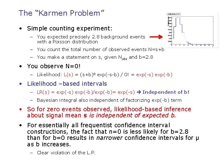
The “Karmen Problem” • Simple counting experiment: – You expected precisely 2. 8 background events with a Poisson distribution – You count the total number of observed events N=s+b – You make a statement on s, given Nobs and b=2. 8 • You observe N=0! – Likelihood: L(s) = (s+b)0 exp(-s-b) / 0! = exp(-s) exp(-b) • Likelihood –based intervals – LR(s) = exp(-s) exp(-b)/exp(-b)= exp(-s) Independent of b! – Bayesian integral also independent of factorizing exp(-b) term • So for zero events observed, likelihood-based inference about signal mean s is independent of expected b. • For essentially all frequentist confidence interval constructions, the fact that n=0 is less likely for b=2. 8 than for b=0 results in narrower confidence intervals for μ as b increases. – Clear violation of the L. P.

Likelihood Principle Example #2 • Binomial problem famous among statisticians • Translated to HEP: You want to know the trigger efficiency e. – You count until reaching n=4000 zero-bias events, and note that of these, m=10 passed trigger. Estimate e = 10/4000, compute binomial conf. interval for e. – Your colleague (in a different sample!) counts zero-bias events until m=10 have passed the trigger. She notes that this requires n=4000 events. Intuitively, e=10/4000 over-estimates e because she stopped just upon reaching 10 passed events. (The relevant distribution is the negative binomial. ) • Each experiment had a different stopping rule. Frequentist confidence intervals depend on the stopping rule. – It turns out that the likelihood functions for the binomial problem and the negative binomial problem differ only by a constant! – So with same n and m, (the strong version of) the L. P. demands same inference about e from the two stopping rules! Wouter Verkerke, NIKHEF [B. Cousins HPCP]

Conditioning • An “ancillary statistic” (see literature for precise math definition) is a function of your data which carries information about the precision of your measurement of the parameter of interest, but no info about parameter’s value. – The classic example is a branching ratio measurement in which the total number of events N can fluctuate if the expt design is to run for a fixed length of time. Then N is an ancillary statistic. • You perform an experiment and obtain N total events, and then do a toy M. C. of repetitions of the experiment. Do you let N fluctuate, or do you fix it to the value observed? • It may seem that the toy M. C. should include your complete procedure, including fluctuations in N. • But there are strong arguments, going back to Fisher, that inference should be based on probabilities conditional on the value of the ancillary statistic actually obtained! Wouter Verkerke, NIKHEF [B. Cousins HPCP]

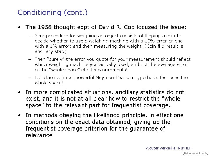
Conditioning (cont. ) • The 1958 thought expt of David R. Cox focused the issue: – Your procedure for weighing an object consists of flipping a coin to decide whether to use a weighing machine with a 10% error or one with a 1% error; and then measuring the weight. (Coin flip result is ancillary stat. ) – Then “surely” the error you quote for your measurement should reflect which weighing machine you actually used, and not the average error of the “whole space” of all measurements! – But classical most powerful Neyman-Pearson hypothesis test uses the whole space! • In more complicated situations, ancillary statistics do not exist, and it is not at all clear how to restrict the “whole space” to the relevant part for frequentist coverage. • In methods obeying the likelihood principle, in effect one conditions on the exact data obtained, giving up the frequentist coverage criterion for the guarantee of relevance Wouter Verkerke, NIKHEF [B. Cousins HPCP]

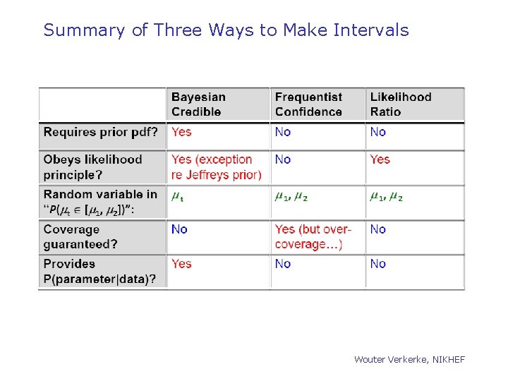
Summary of Three Ways to Make Intervals Wouter Verkerke, NIKHEF

68% intervals by various methods for Poisson process with n=3 observed • NB: Frequentist intervals over-cover due to discreteness of n in this example • Note that issues, divergences in outcome are usually more dramatic and important at high Z (e. g. 5σ = ‘discovery’) Wouter Verkerke, NIKHEF [B. Cousins HPCP]

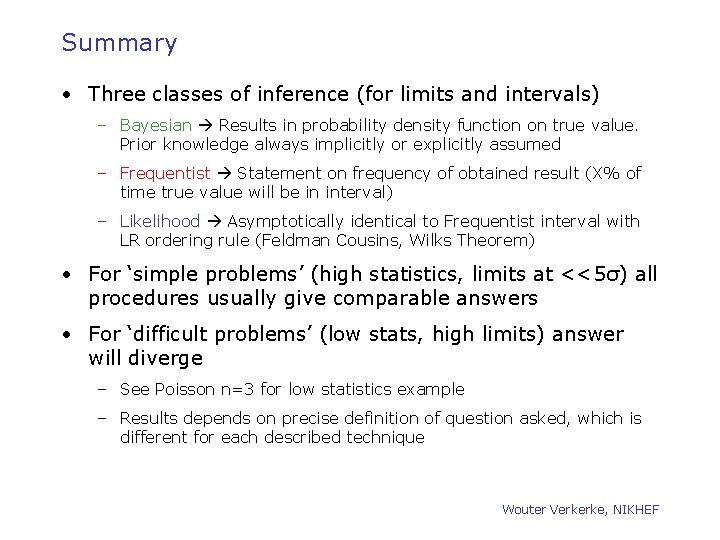
Summary • Three classes of inference (for limits and intervals) – Bayesian Results in probability density function on true value. Prior knowledge always implicitly or explicitly assumed – Frequentist Statement on frequency of obtained result (X% of time true value will be in interval) – Likelihood Asymptotically identical to Frequentist interval with LR ordering rule (Feldman Cousins, Wilks Theorem) • For ‘simple problems’ (high statistics, limits at <<5σ) all procedures usually give comparable answers • For ‘difficult problems’ (low stats, high limits) answer will diverge – See Poisson n=3 for low statistics example – Results depends on precise definition of question asked, which is different for each described technique Wouter Verkerke, NIKHEF