Chapter 6 Hypothesis Testing What is Hypothesis Testing

Chapter 6 Hypothesis Testing

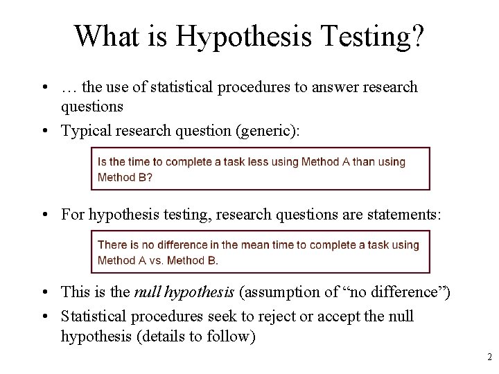
What is Hypothesis Testing? • … the use of statistical procedures to answer research questions • Typical research question (generic): • For hypothesis testing, research questions are statements: • This is the null hypothesis (assumption of “no difference”) • Statistical procedures seek to reject or accept the null hypothesis (details to follow) 2

Statistical Procedures • Two types: – Parametric • Data are assumed to come from a distribution, such as the normal distribution, t-distribution, etc. – Non-parametric • Data are not assumed to come from a distribution – Lots of debate on assumptions testing and what to do if assumptions are not met (avoided here, for the most part) – A reasonable basis for deciding on the most appropriate test is to match the type of test with the measurement scale of the data (next slide) 3

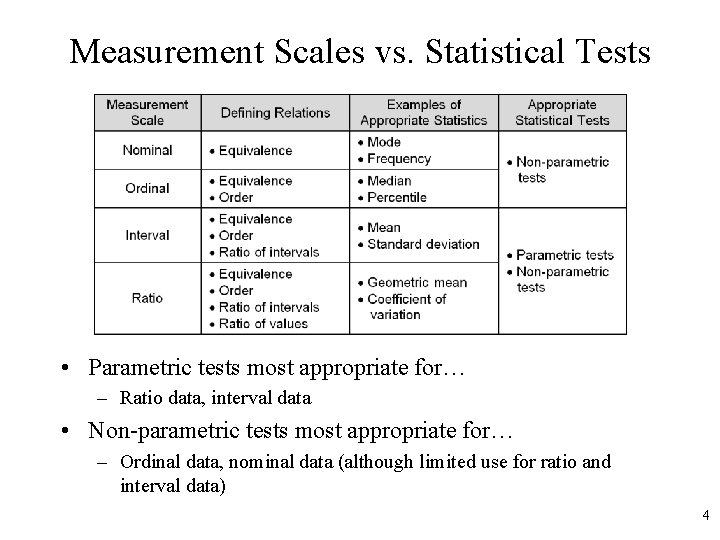
Measurement Scales vs. Statistical Tests • Parametric tests most appropriate for… – Ratio data, interval data • Non-parametric tests most appropriate for… – Ordinal data, nominal data (although limited use for ratio and interval data) 4

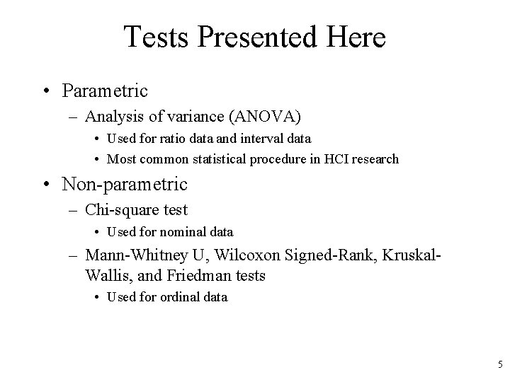
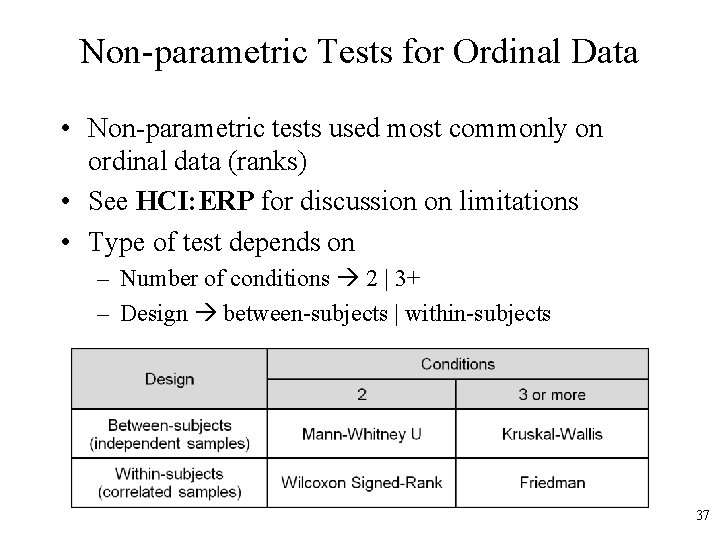
Tests Presented Here • Parametric – Analysis of variance (ANOVA) • Used for ratio data and interval data • Most common statistical procedure in HCI research • Non-parametric – Chi-square test • Used for nominal data – Mann-Whitney U, Wilcoxon Signed-Rank, Kruskal. Wallis, and Friedman tests • Used for ordinal data 5

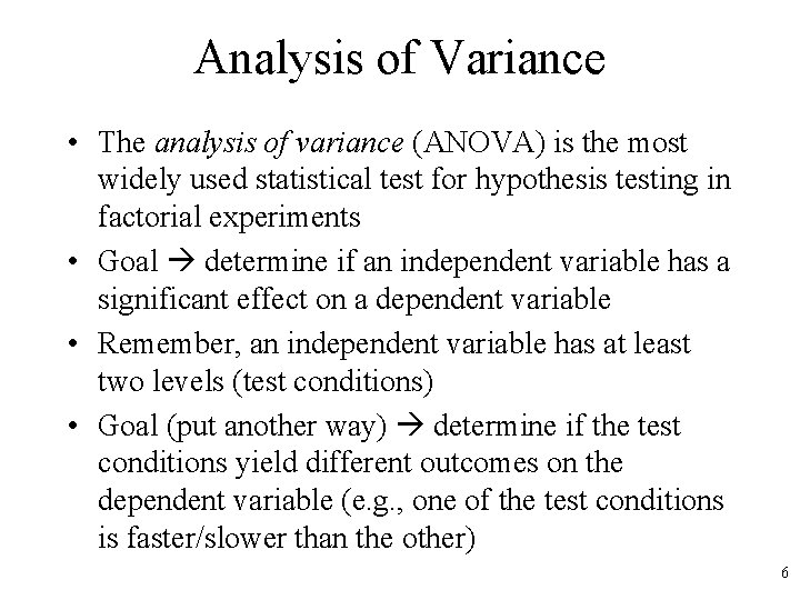
Analysis of Variance • The analysis of variance (ANOVA) is the most widely used statistical test for hypothesis testing in factorial experiments • Goal determine if an independent variable has a significant effect on a dependent variable • Remember, an independent variable has at least two levels (test conditions) • Goal (put another way) determine if the test conditions yield different outcomes on the dependent variable (e. g. , one of the test conditions is faster/slower than the other) 6

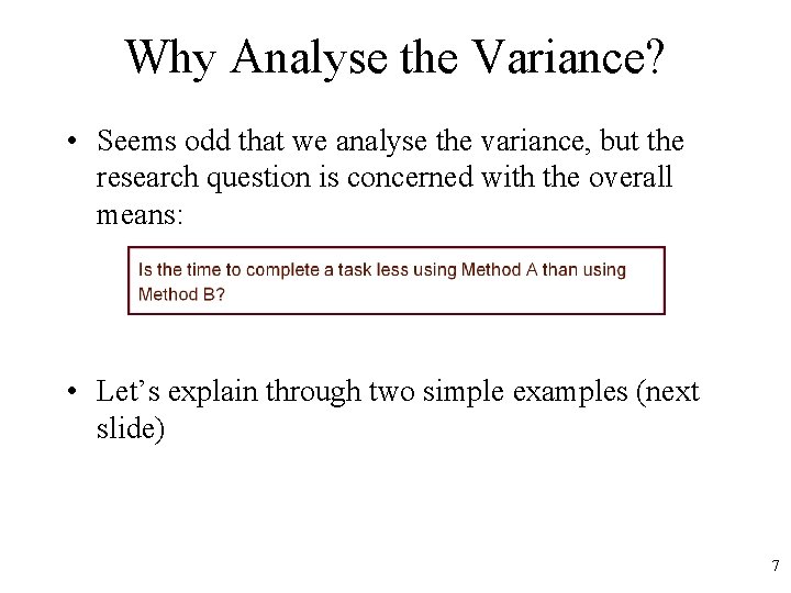
Why Analyse the Variance? • Seems odd that we analyse the variance, but the research question is concerned with the overall means: • Let’s explain through two simple examples (next slide) 7

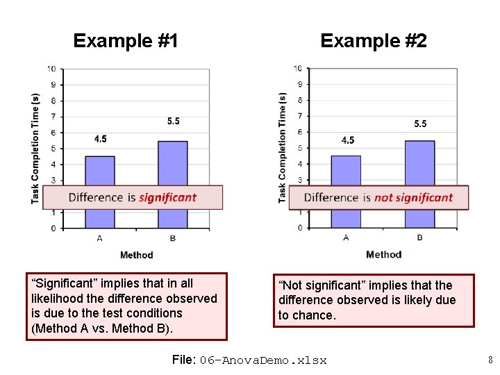
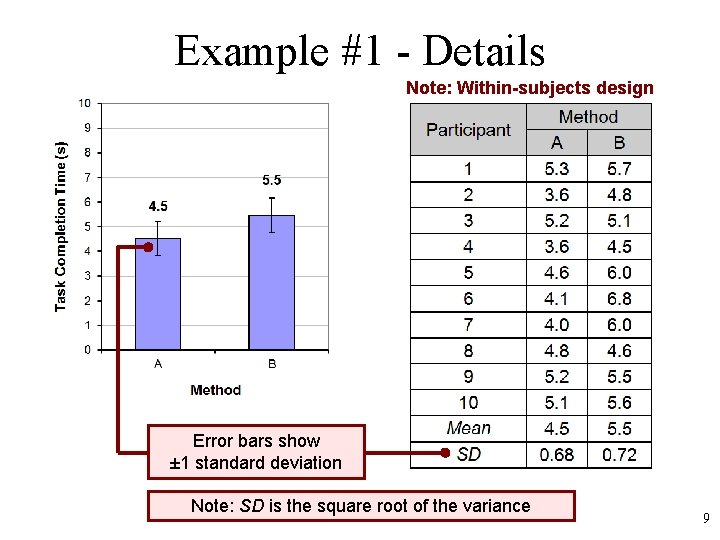
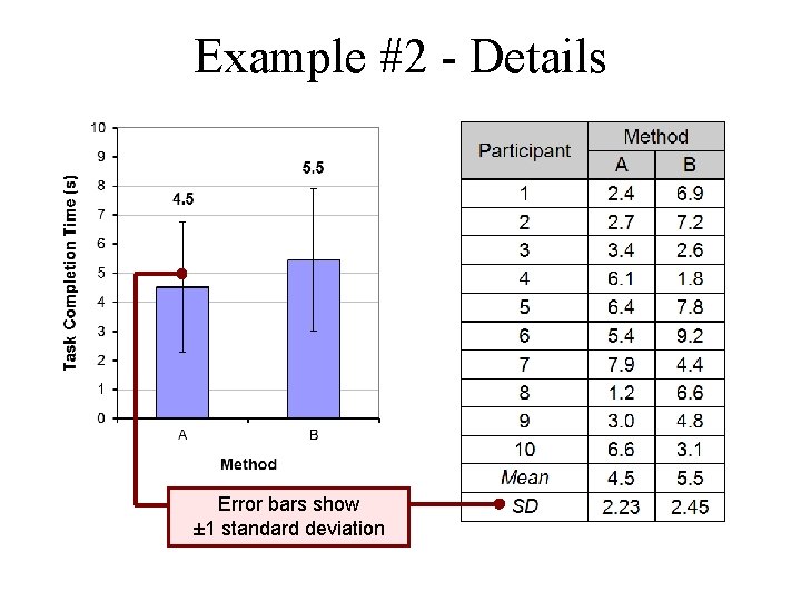
Example #1 “Significant” implies that in all likelihood the difference observed is due to the test conditions (Method A vs. Method B). Example #2 “Not significant” implies that the difference observed is likely due to chance. File: 06 -Anova. Demo. xlsx 8

Example #1 - Details Note: Within-subjects design Error bars show ± 1 standard deviation Note: SD is the square root of the variance 9

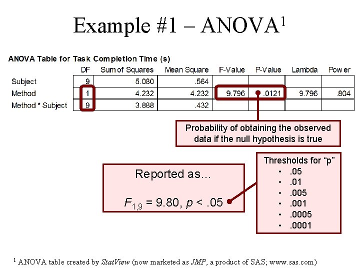
Example #1 – ANOVA 1 Probability of obtaining the observed data if the null hypothesis is true Reported as… F 1, 9 = 9. 80, p <. 05 1 Thresholds for “p” • . 05 • . 01 • . 005 • . 001 • . 0005 • . 0001 ANOVA table created by Stat. View (now marketed as JMP, a product of SAS; www. sas. com)

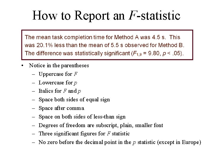
How to Report an F-statistic • Notice in the parentheses – Uppercase for F – Lowercase for p – Italics for F and p – Space both sides of equal sign – Space after comma – Space on both sides of less-than sign – Degrees of freedom are subscript, plain, smaller font – Three significant figures for F statistic – No zero before the decimal point in the p statistic (except in Europe)

Example #2 - Details Error bars show ± 1 standard deviation

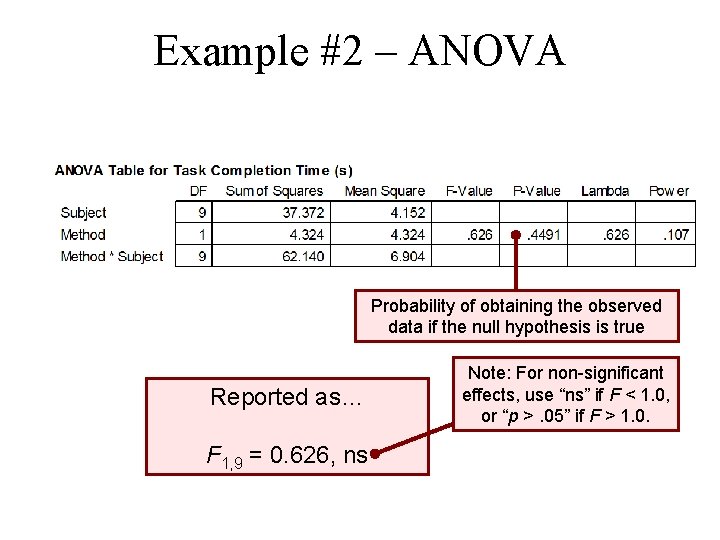
Example #2 – ANOVA Probability of obtaining the observed data if the null hypothesis is true Reported as… F 1, 9 = 0. 626, ns Note: For non-significant effects, use “ns” if F < 1. 0, or “p >. 05” if F > 1. 0.

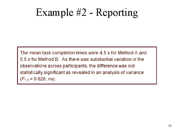
Example #2 - Reporting 14

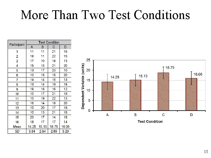
More Than Two Test Conditions 15

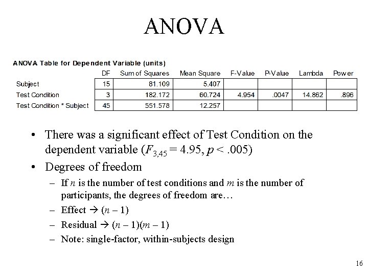
ANOVA • There was a significant effect of Test Condition on the dependent variable (F 3, 45 = 4. 95, p <. 005) • Degrees of freedom – If n is the number of test conditions and m is the number of participants, the degrees of freedom are… – Effect (n – 1) – Residual (n – 1)(m – 1) – Note: single-factor, within-subjects design 16

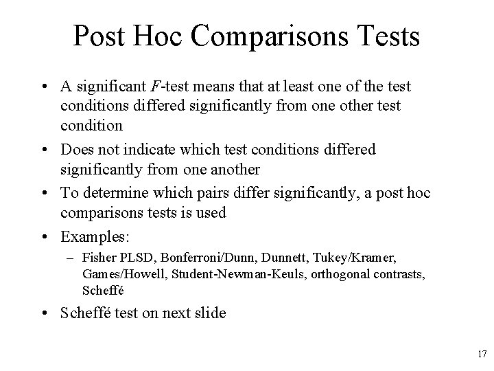
Post Hoc Comparisons Tests • A significant F-test means that at least one of the test conditions differed significantly from one other test condition • Does not indicate which test conditions differed significantly from one another • To determine which pairs differ significantly, a post hoc comparisons tests is used • Examples: – Fisher PLSD, Bonferroni/Dunn, Dunnett, Tukey/Kramer, Games/Howell, Student-Newman-Keuls, orthogonal contrasts, Scheffé • Scheffé test on next slide 17

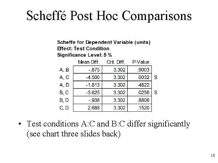
Scheffé Post Hoc Comparisons • Test conditions A: C and B: C differ significantly (see chart three slides back) 18

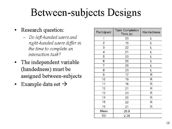
Between-subjects Designs • Research question: – Do left-handed users and right-handed users differ in the time to complete an interaction task? • The independent variable (handedness) must be assigned between-subjects • Example data set 19

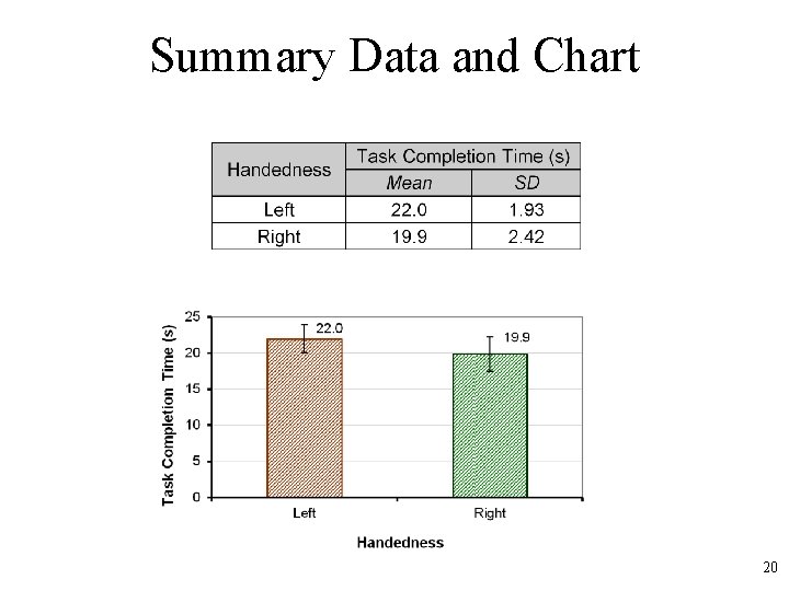
Summary Data and Chart 20

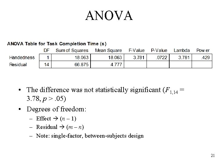
ANOVA • The difference was not statistically significant (F 1, 14 = 3. 78, p >. 05) • Degrees of freedom: – Effect (n – 1) – Residual (m – n) – Note: single-factor, between-subjects design 21

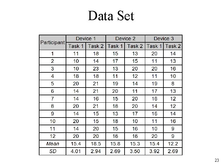
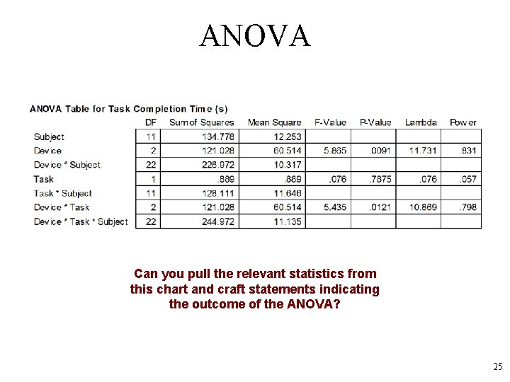
Two-way ANOVA • An experiment with two independent variables is a twoway design • ANOVA tests for – Two main effects + one interaction effect • Example – Independent variables • Device D 1, D 2, D 3 (e. g. , mouse, stylus, touchpad) • Task T 1, T 2 (e. g. , point-select, drag-select) – Dependent variable • Task completion time (or something, this isn’t important here) – Both IVs assigned within-subjects – Participants: 12 – Data set (next slide) 22

Data Set 23

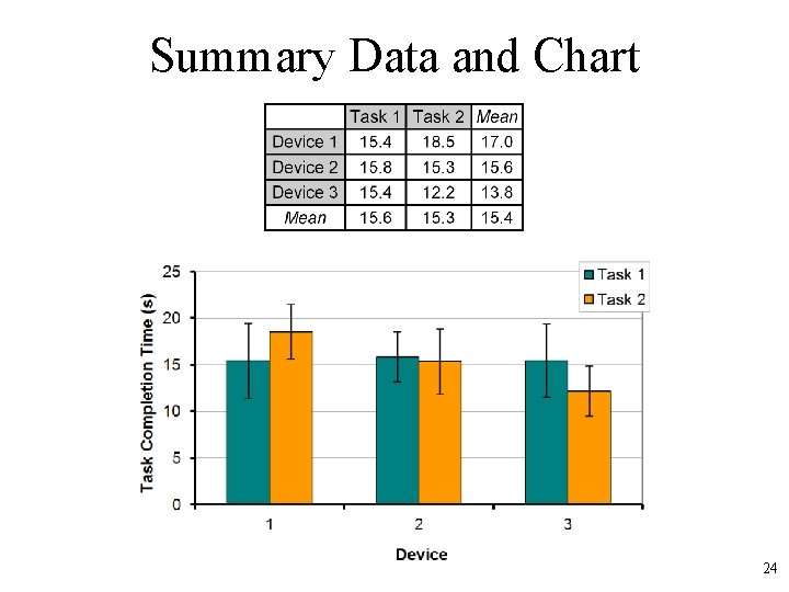
Summary Data and Chart 24

ANOVA Can you pull the relevant statistics from this chart and craft statements indicating the outcome of the ANOVA? 25

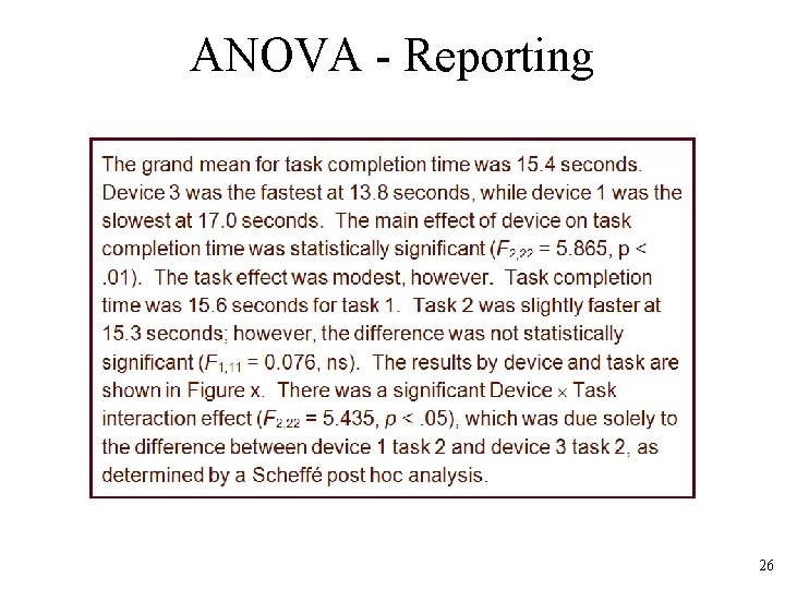
ANOVA - Reporting 26

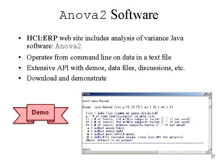
Anova 2 Software • HCI: ERP web site includes analysis of variance Java software: Anova 2 • Operates from command line on data in a text file • Extensive API with demos, data files, discussions, etc. • Download and demonstrate Demo 27

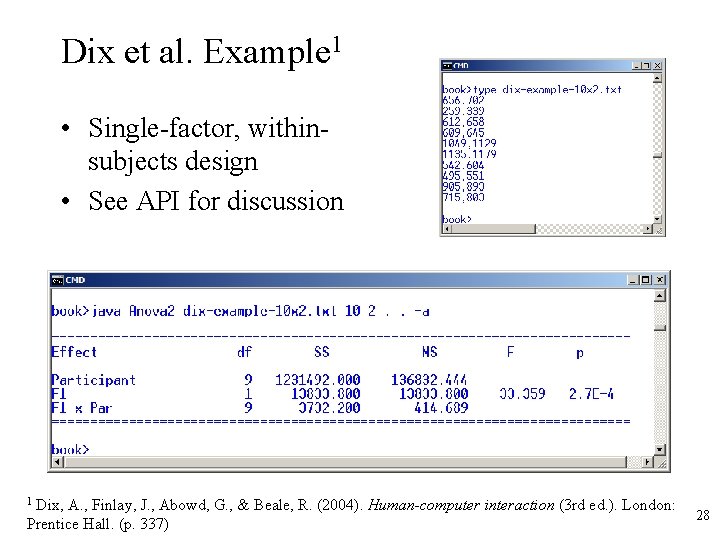
Dix et al. Example 1 • Single-factor, withinsubjects design • See API for discussion Dix, A. , Finlay, J. , Abowd, G. , & Beale, R. (2004). Human-computer interaction (3 rd ed. ). London: Prentice Hall. (p. 337) 1 28

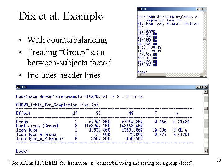
Dix et al. Example • With counterbalancing • Treating “Group” as a between-subjects factor 1 • Includes header lines 1 See API and HCI: ERP for discussion on “counterbalancing and testing for a group effect”. 29

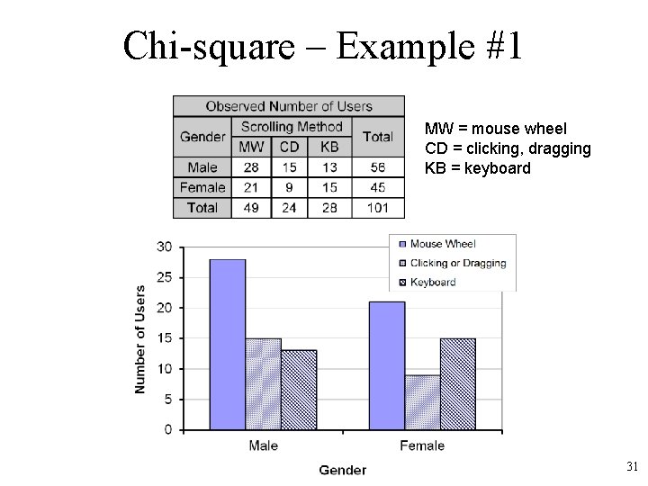
Chi-square Test (Nominal Data) • A chi-square test is used to investigate relationships • Relationships between categorical, or nominal-scale, variables representing attributes of people, interaction techniques, systems, etc. • Data organized in a contingency table – cross tabulation containing counts (frequency data) for number of observations in each category • A chi-square test compares the observed values against expected values • Expected values assume “no difference” • Research question: – Do males and females differ in their method of scrolling on desktop systems? (next slide) 30

Chi-square – Example #1 MW = mouse wheel CD = clicking, dragging KB = keyboard 31

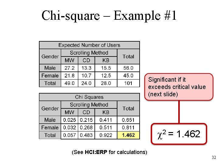
Chi-square – Example #1 Significant if it exceeds critical value (next slide) 2 = 1. 462 (See HCI: ERP for calculations) 32

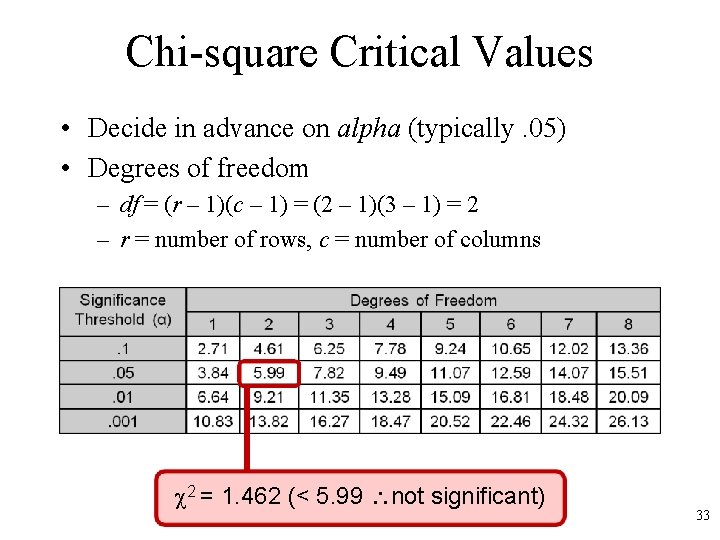
Chi-square Critical Values • Decide in advance on alpha (typically. 05) • Degrees of freedom – df = (r – 1)(c – 1) = (2 – 1)(3 – 1) = 2 – r = number of rows, c = number of columns 2 = 1. 462 (< 5. 99 not significant) 33

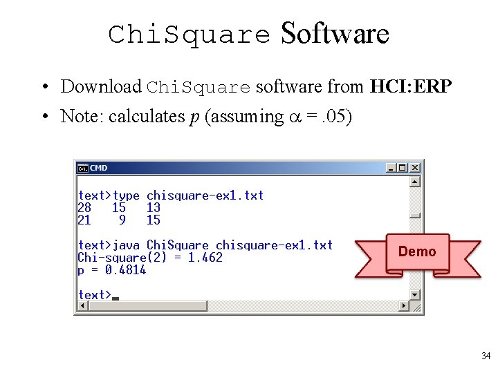
Chi. Square Software • Download Chi. Square software from HCI: ERP • Note: calculates p (assuming =. 05) Demo 34

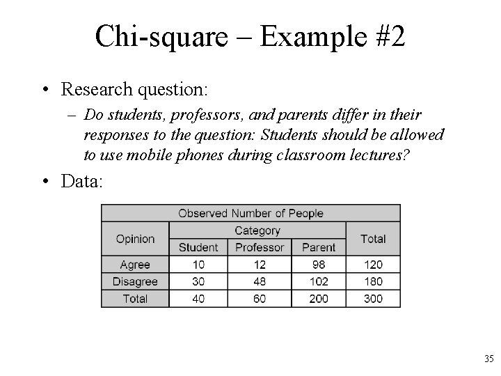
Chi-square – Example #2 • Research question: – Do students, professors, and parents differ in their responses to the question: Students should be allowed to use mobile phones during classroom lectures? • Data: 35

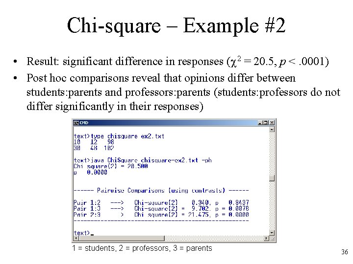
Chi-square – Example #2 • Result: significant difference in responses ( 2 = 20. 5, p <. 0001) • Post hoc comparisons reveal that opinions differ between students: parents and professors: parents (students: professors do not differ significantly in their responses) 1 = students, 2 = professors, 3 = parents 36

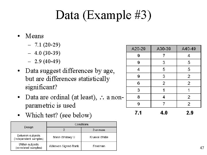
Non-parametric Tests for Ordinal Data • Non-parametric tests used most commonly on ordinal data (ranks) • See HCI: ERP for discussion on limitations • Type of test depends on – Number of conditions 2 | 3+ – Design between-subjects | within-subjects 37

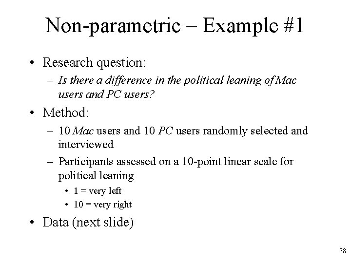
Non-parametric – Example #1 • Research question: – Is there a difference in the political leaning of Mac users and PC users? • Method: – 10 Mac users and 10 PC users randomly selected and interviewed – Participants assessed on a 10 -point linear scale for political leaning • 1 = very left • 10 = very right • Data (next slide) 38

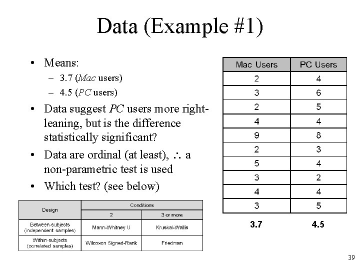
Data (Example #1) • Means: – 3. 7 (Mac users) – 4. 5 (PC users) • Data suggest PC users more rightleaning, but is the difference statistically significant? • Data are ordinal (at least), a non-parametric test is used • Which test? (see below) 3. 7 4. 5 39

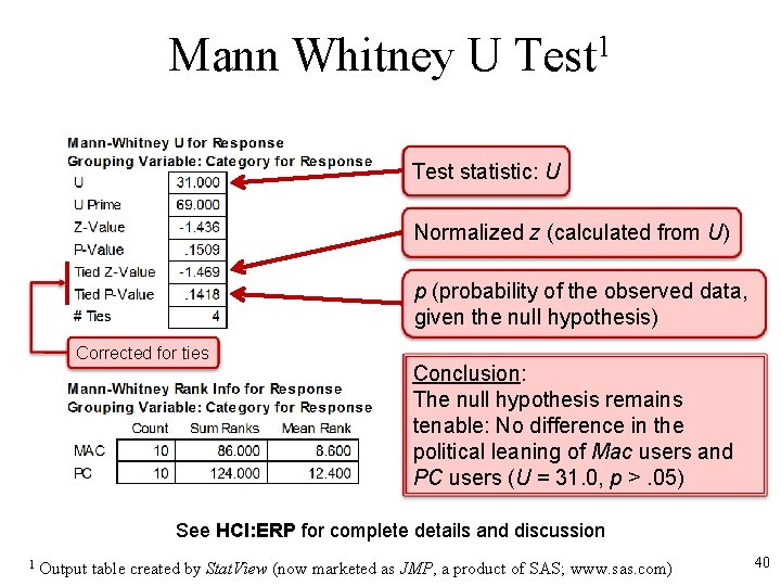
Mann Whitney U Test 1 Test statistic: U Normalized z (calculated from U) p (probability of the observed data, given the null hypothesis) Corrected for ties Conclusion: The null hypothesis remains tenable: No difference in the political leaning of Mac users and PC users (U = 31. 0, p >. 05) See HCI: ERP for complete details and discussion 1 Output table created by Stat. View (now marketed as JMP, a product of SAS; www. sas. com) 40

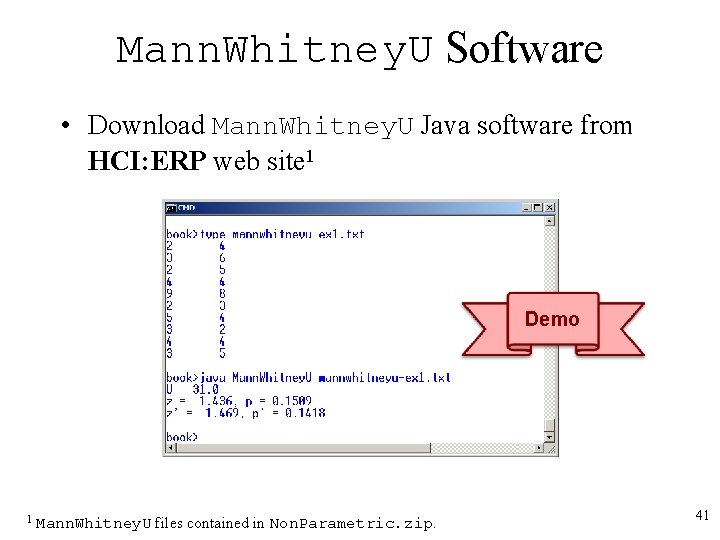
Mann. Whitney. U Software • Download Mann. Whitney. U Java software from HCI: ERP web site 1 Demo 1 Mann. Whitney. U files contained in Non. Parametric. zip. 41

Non-parametric – Example #2 • Research question: – Do two new designs for media players differ in “cool appeal” for young users? • Method: – 10 young tech-savvy participants recruited and given demos of the two media players (MPA, MPB) – Participants asked to rate the media players for “cool appeal” on a 10 -point linear scale • 1 = not cool at all • 10 = really cool • Data (next slide) 42

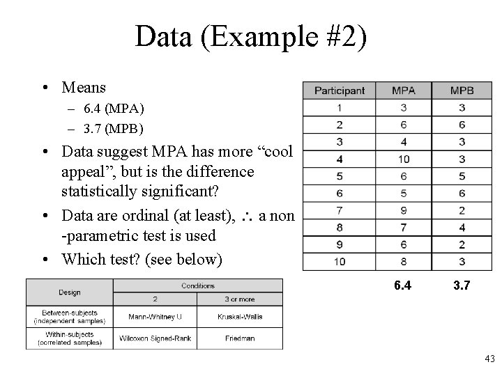
Data (Example #2) • Means – 6. 4 (MPA) – 3. 7 (MPB) • Data suggest MPA has more “cool appeal”, but is the difference statistically significant? • Data are ordinal (at least), a non -parametric test is used • Which test? (see below) 6. 4 3. 7 43

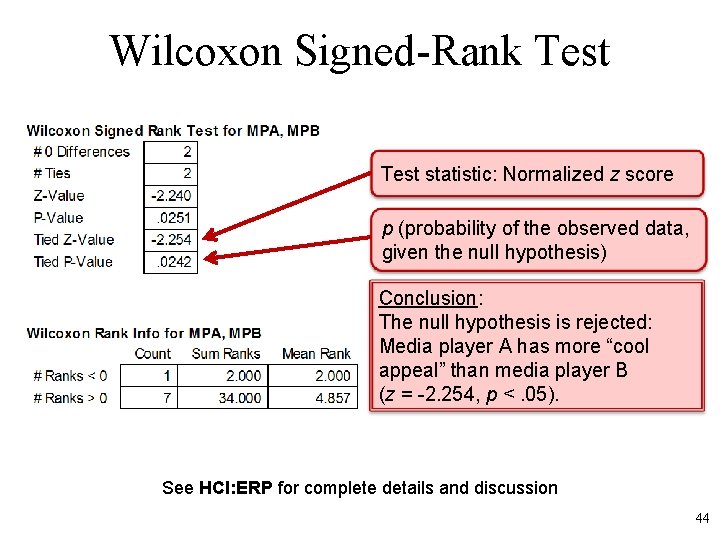
Wilcoxon Signed-Rank Test statistic: Normalized z score p (probability of the observed data, given the null hypothesis) Conclusion: The null hypothesis is rejected: Media player A has more “cool appeal” than media player B (z = -2. 254, p <. 05). See HCI: ERP for complete details and discussion 44

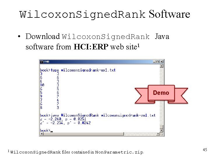
Wilcoxon. Signed. Rank Software • Download Wilcoxon. Signed. Rank Java software from HCI: ERP web site 1 Demo 1 Wilcoxon. Signed. Rank files contained in Non. Parametric. zip. 45

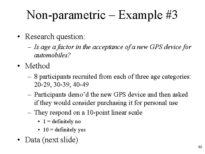
Non-parametric – Example #3 • Research question: – Is age a factor in the acceptance of a new GPS device for automobiles? • Method – 8 participants recruited from each of three age categories: 20 -29, 30 -39, 40 -49 – Participants demo’d the new GPS device and then asked if they would consider purchasing it for personal use – They respond on a 10 -point linear scale • 1 = definitely no • 10 = definitely yes • Data (next slide) 46

Data (Example #3) • Means – 7. 1 (20 -29) – 4. 0 (30 -39) – 2. 9 (40 -49) • Data suggest differences by age, but are differences statistically significant? • Data are ordinal (at least), a nonparametric is used • Which test? (see below) 7. 1 4. 0 2. 9 47

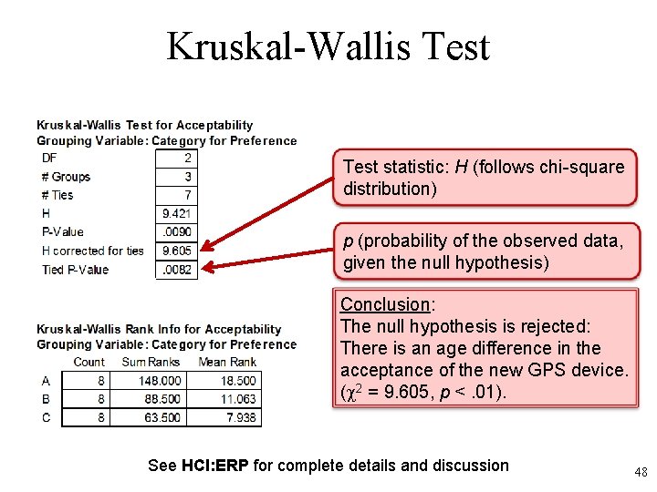
Kruskal-Wallis Test statistic: H (follows chi-square distribution) p (probability of the observed data, given the null hypothesis) Conclusion: The null hypothesis is rejected: There is an age difference in the acceptance of the new GPS device. ( 2 = 9. 605, p <. 01). See HCI: ERP for complete details and discussion 48

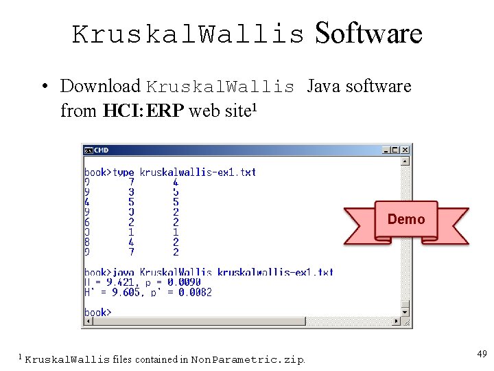
Kruskal. Wallis Software • Download Kruskal. Wallis Java software from HCI: ERP web site 1 Demo 1 Kruskal. Wallis files contained in Non. Parametric. zip. 49

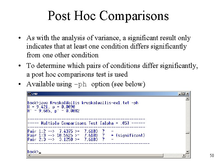
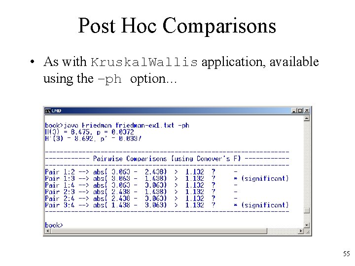
Post Hoc Comparisons • As with the analysis of variance, a significant result only indicates that at least one condition differs significantly from one other condition • To determine which pairs of conditions differ significantly, a post hoc comparisons test is used • Available using –ph option (see below) 50

Non-parametric – Example #4 • Research question: – Do four variations of a search engine interface (A, B, C, D) differ in “quality of results”? • Method – 8 participants recruited and demo’d the four interfaces – Participants do a series of search tasks on the four search interfaces (Note: counterbalancing is used, but this isn’t important here) – Quality of results for each search interface assessed on a linear scale from 1 to 100 • 1 = very poor quality of results • 100 = very good quality of results • Data (next slide) 51

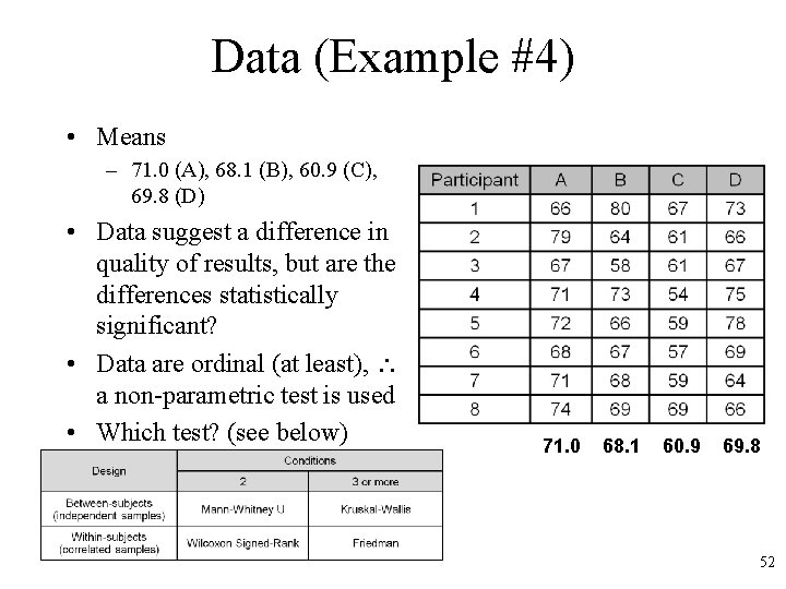
Data (Example #4) • Means – 71. 0 (A), 68. 1 (B), 60. 9 (C), 69. 8 (D) • Data suggest a difference in quality of results, but are the differences statistically significant? • Data are ordinal (at least), a non-parametric test is used • Which test? (see below) 71. 0 68. 1 60. 9 69. 8 52

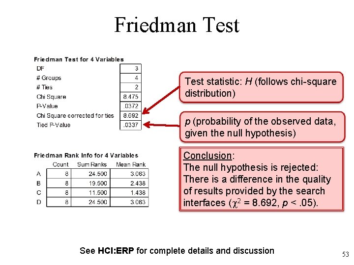
Friedman Test statistic: H (follows chi-square distribution) p (probability of the observed data, given the null hypothesis) Conclusion: The null hypothesis is rejected: There is a difference in the quality of results provided by the search interfaces ( 2 = 8. 692, p <. 05). See HCI: ERP for complete details and discussion 53

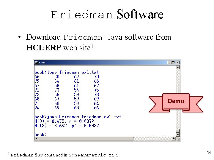
Friedman Software • Download Friedman Java software from HCI: ERP web site 1 Demo 1 Friedman files contained in Non. Parametric. zip. 54

Post Hoc Comparisons • As with Kruskal. Wallis application, available using the –ph option… 55

Points of Discussion • Reporting the mean vs. median for scaled responses • Non-parametric tests for multi-factor experiments • Non-parametric tests for ratio-scale data See HCI: ERP for complete details and discussion 56

Thank You 57