Pearsons r 2 X Correlation vs X which

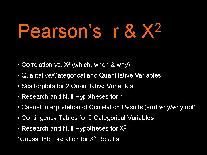
Pearson’s r & 2 X • Correlation vs. X² (which, when & why) • Qualitative/Categorical and Quantitative Variables • Scatterplots for 2 Quantitative Variables • Research and Null Hypotheses for r • Casual Interpretation of Correlation Results (and why/why not) • Contingency Tables for 2 Categorical Variables • Research and Null Hypotheses for X 2 • Causal Interpretation for X 2 Results

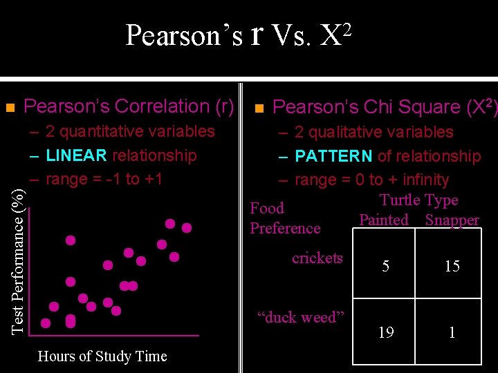
Pearson’s r Vs. n Pearson’s Correlation (r) Test Performance (%) – 2 quantitative variables – LINEAR relationship – range = -1 to +1 n 2 X Pearson’s Chi Square (X 2) – 2 qualitative variables – PATTERN of relationship – range = 0 to + infinity Turtle Type Food Painted Snapper Preference crickets “duck weed” Hours of Study Time 5 15 19 1

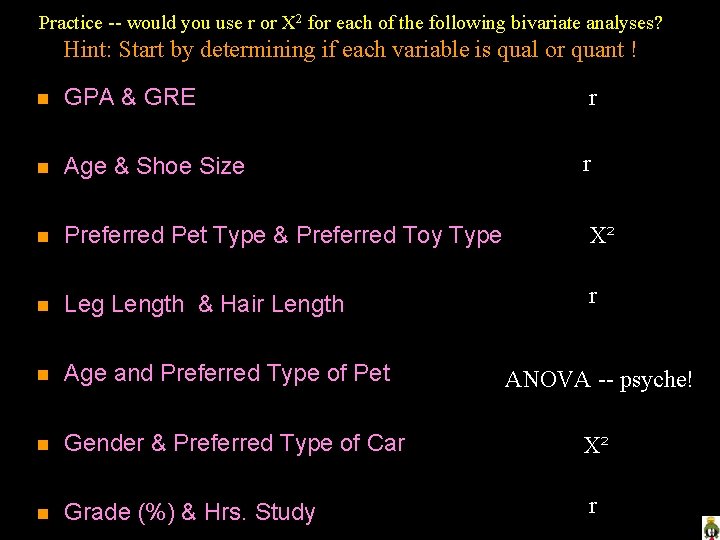
Practice -- would you use r or X 2 for each of the following bivariate analyses? Hint: Start by determining if each variable is qual or quant ! n GPA & GRE r n Age & Shoe Size r n Preferred Pet Type & Preferred Toy Type X² n Leg Length & Hair Length r n Age and Preferred Type of Pet n Gender & Preferred Type of Car X² n Grade (%) & Hrs. Study r ANOVA -- psyche!

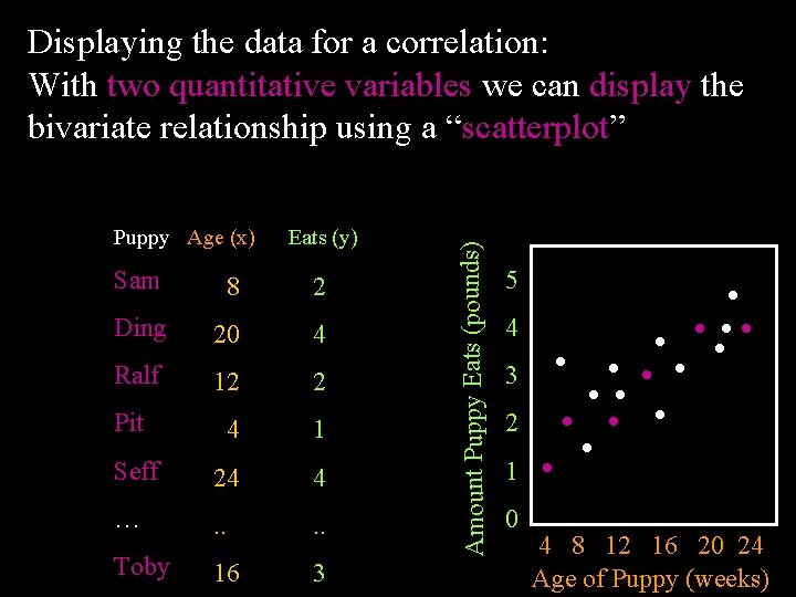
Puppy Age (x) Eats (y) Sam 8 2 Ding 20 4 Ralf 12 2 Pit 4 1 Seff 24 4 … . . Toby 16 3 Amount Puppy Eats (pounds) Displaying the data for a correlation: With two quantitative variables we can display the bivariate relationship using a “scatterplot” 5 4 3 2 1 0 4 8 12 16 20 24 Age of Puppy (weeks)

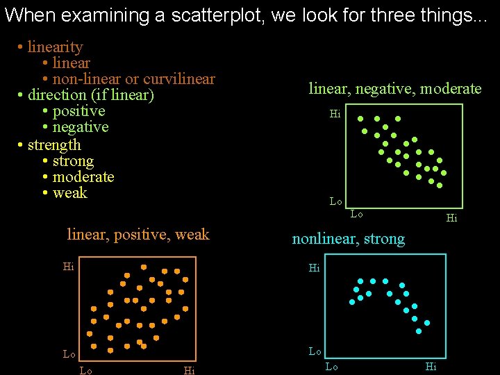
When examining a scatterplot, we look for three things. . . • linearity • linear • non-linear or curvilinear • direction (if linear) • positive • negative • strength • strong • moderate • weak linear, negative, moderate Hi Lo Lo linear, positive, weak nonlinear, strong Hi Hi Lo Lo Lo Hi Hi Lo Hi

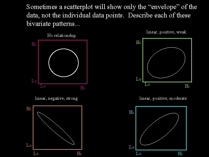
Sometimes a scatterplot will show only the “envelope” of the data, not the individual data points. Describe each of these bivariate patterns. . . linear, positive, weak No relationship Hi Hi Lo Lo Hi linear, negative, strong Hi Hi linear, positive, moderate Hi Lo Lo Lo Hi

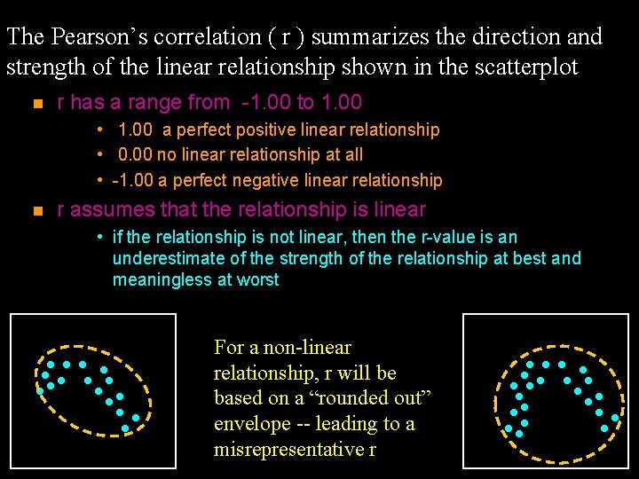
The Pearson’s correlation ( r ) summarizes the direction and strength of the linear relationship shown in the scatterplot n r has a range from -1. 00 to 1. 00 • 1. 00 a perfect positive linear relationship • 0. 00 no linear relationship at all • -1. 00 a perfect negative linear relationship n r assumes that the relationship is linear • if the relationship is not linear, then the r-value is an underestimate of the strength of the relationship at best and meaningless at worst For a non-linear relationship, r will be based on a “rounded out” envelope -- leading to a misrepresentative r

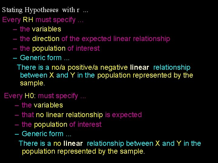
Stating Hypotheses with r. . . Every RH must specify. . . – the variables – the direction of the expected linear relationship – the population of interest – Generic form. . . There is a no/a positive/a negative linear relationship between X and Y in the population represented by the sample. Every H 0: must specify. . . – the variables – that no linear relationship is expected – the population of interest – Generic form. . . There is a no linear relationship between X and Y in the population represented by the sample.

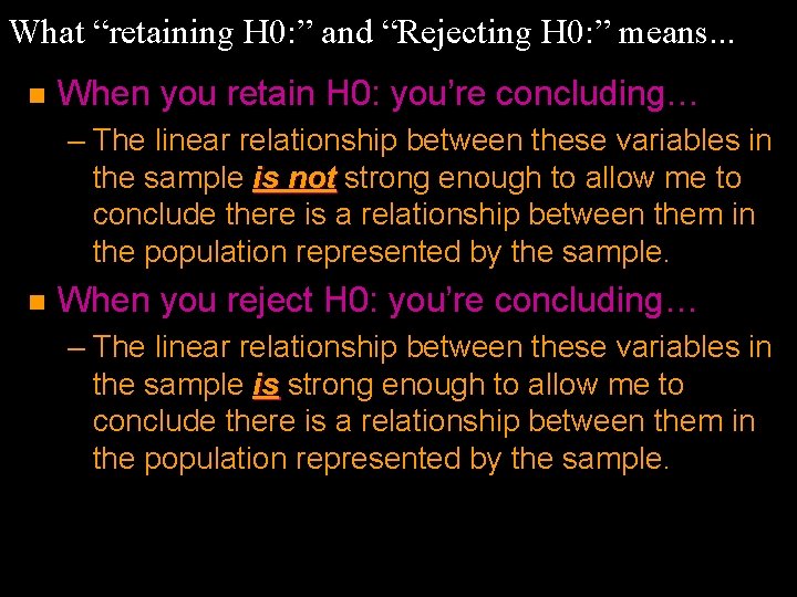
What “retaining H 0: ” and “Rejecting H 0: ” means. . . n When you retain H 0: you’re concluding… – The linear relationship between these variables in the sample is not strong enough to allow me to conclude there is a relationship between them in the population represented by the sample. n When you reject H 0: you’re concluding… – The linear relationship between these variables in the sample is strong enough to allow me to conclude there is a relationship between them in the population represented by the sample.

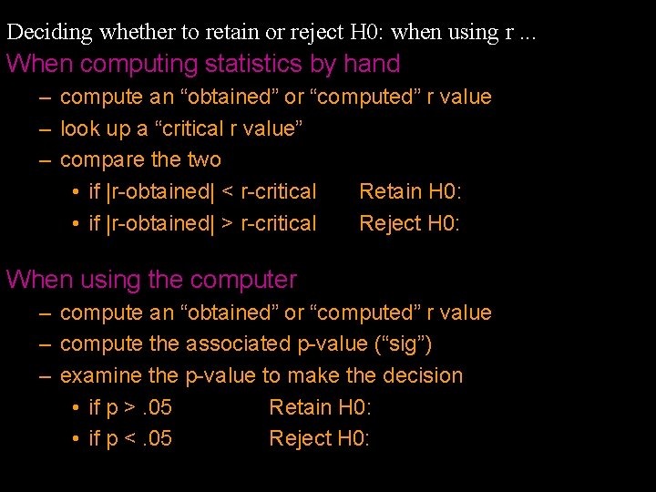
Deciding whether to retain or reject H 0: when using r. . . When computing statistics by hand – compute an “obtained” or “computed” r value – look up a “critical r value” – compare the two • if |r-obtained| < r-critical Retain H 0: • if |r-obtained| > r-critical Reject H 0: When using the computer – compute an “obtained” or “computed” r value – compute the associated p-value (“sig”) – examine the p-value to make the decision • if p >. 05 Retain H 0: • if p <. 05 Reject H 0:

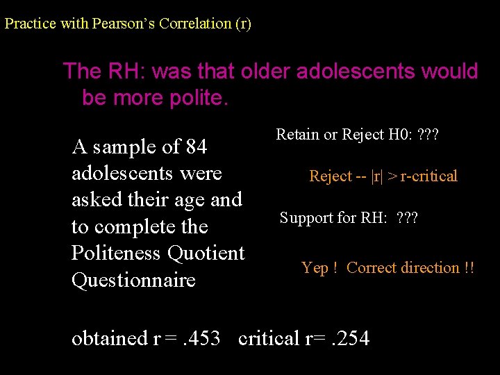
Practice with Pearson’s Correlation (r) The RH: was that older adolescents would be more polite. A sample of 84 adolescents were asked their age and to complete the Politeness Quotient Questionnaire Retain or Reject H 0: ? ? ? Reject -- |r| > r-critical Support for RH: ? ? ? Yep ! Correct direction !! obtained r =. 453 critical r=. 254

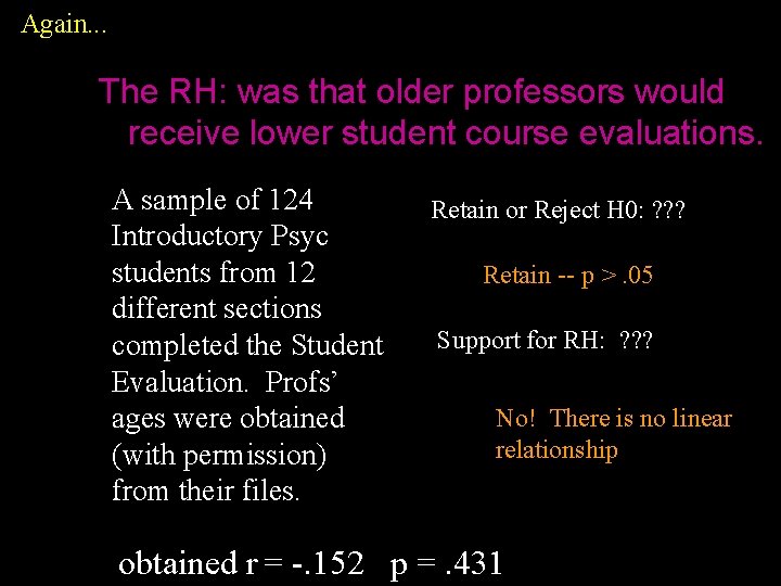
Again. . . The RH: was that older professors would receive lower student course evaluations. A sample of 124 Introductory Psyc students from 12 different sections completed the Student Evaluation. Profs’ ages were obtained (with permission) from their files. Retain or Reject H 0: ? ? ? Retain -- p >. 05 Support for RH: ? ? ? No! There is no linear relationship obtained r = -. 152 p =. 431

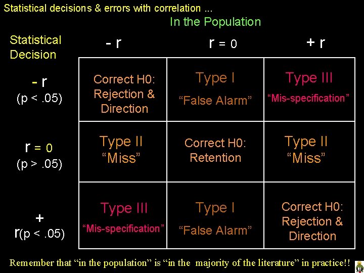
Statistical decisions & errors with correlation. . . In the Population Statistical Decision -r -r r=0 Type III “False Alarm” “Mis-specification” Type II “Miss” (p <. 05) Correct H 0: Rejection & Direction r=0 Type II “Miss” Correct H 0: Retention Type III Type I “Mis-specification” “False Alarm” (p >. 05) + r(p <. 05) +r Correct H 0: Rejection & Direction Remember that “in the population” is “in the majority of the literature” in practice!!

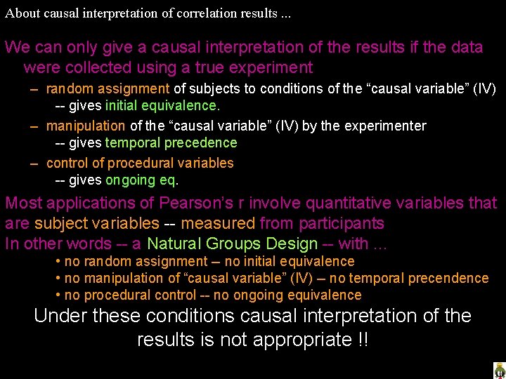
About causal interpretation of correlation results. . . We can only give a causal interpretation of the results if the data were collected using a true experiment – random assignment of subjects to conditions of the “causal variable” (IV) -- gives initial equivalence. – manipulation of the “causal variable” (IV) by the experimenter -- gives temporal precedence – control of procedural variables -- gives ongoing eq. Most applications of Pearson’s r involve quantitative variables that are subject variables -- measured from participants In other words -- a Natural Groups Design -- with. . . • no random assignment -- no initial equivalence • no manipulation of “causal variable” (IV) -- no temporal precendence • no procedural control -- no ongoing equivalence Under these conditions causal interpretation of the results is not appropriate !!

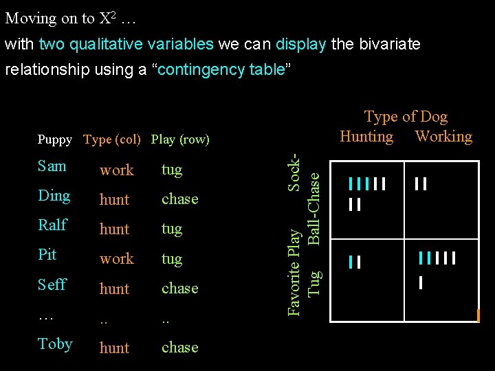
Moving on to X 2 … with two qualitative variables we can display the bivariate relationship using a “contingency table” Type of Dog Hunting Working Sam work tug Ding hunt chase Ralf hunt tug Pit work tug Seff hunt chase … . . Toby hunt chase Favorite Play Sock. Tug Ball-Chase Puppy Type (col) Play (row)

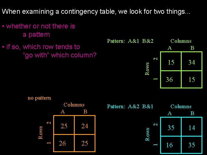
When examining a contingency table, we look for two things. . . 2 Columns A B 15 34 36 15 Rows • if so, which row tends to “go with” which column? Pattern: A&1 B&2 1 • whether or not there is a pattern no pattern 2 25 Columns A B 35 14 1 26 Pattern: A&2 B&1 16 35 Rows 2 24 Rows 25 1 Columns A B

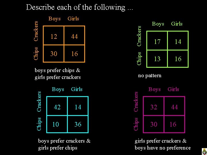
44 30 16 Chips Crackers boys prefer chips & girls prefer crackers Boys Girls 42 14 10 36 boys prefer crackers & girls prefer chips Crackers 12 Chips Girls Boys Girls 17 14 13 16 no pattern Crackers Boys Chips Crackers Describe each of the following. . . Boys Girls 32 44 30 16 girls prefer crackers & boys have no preference

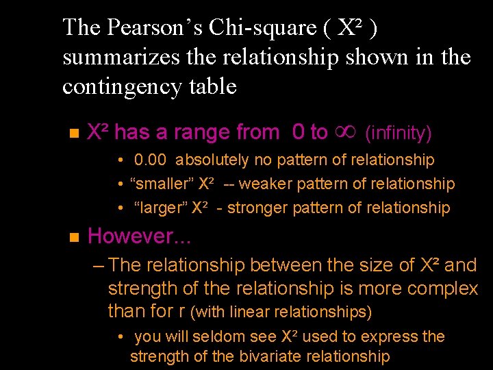
The Pearson’s Chi-square ( X² ) summarizes the relationship shown in the contingency table n X² has a range from 0 to (infinity) • 0. 00 absolutely no pattern of relationship • “smaller” X² -- weaker pattern of relationship • “larger” X² - stronger pattern of relationship n However. . . – The relationship between the size of X² and strength of the relationship is more complex than for r (with linear relationships) • you will seldom see X² used to express the strength of the bivariate relationship

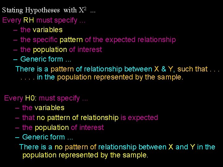
Stating Hypotheses with X 2. . . Every RH must specify. . . – the variables – the specific pattern of the expected relationship – the population of interest – Generic form. . . There is a pattern of relationship between X & Y, such that. . . . in the population represented by the sample. Every H 0: must specify. . . – the variables – that no pattern of relationship is expected – the population of interest – Generic form. . . There is a no pattern of relationship between X and Y in the population represented by the sample.

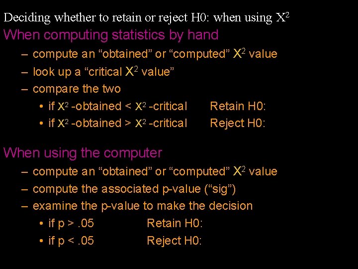
Deciding whether to retain or reject H 0: when using X 2 When computing statistics by hand – compute an “obtained” or “computed” X 2 value – look up a “critical X 2 value” – compare the two • if X 2 -obtained < X 2 -critical Retain H 0: • if X 2 -obtained > X 2 -critical Reject H 0: When using the computer – compute an “obtained” or “computed” X 2 value – compute the associated p-value (“sig”) – examine the p-value to make the decision • if p >. 05 Retain H 0: • if p <. 05 Reject H 0:

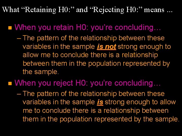
What “Retaining H 0: ” and “Rejecting H 0: ” means. . . n When you retain H 0: you’re concluding… – The pattern of the relationship between these variables in the sample is not strong enough to allow me to conclude there is a relationship between them in the population represented by the sample. n When you reject H 0: you’re concluding… – The pattern of the relationship between these variables in the sample is strong enough to allow me to conclude there is a relationship between them in the population represented by the sample.

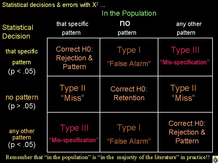
Statistical decisions & errors with X 2. . . In the Population Statistical Decision that specific pattern (p <. 05) no pattern (p >. 05) any other pattern (p <. 05) that specific pattern no pattern any other pattern Correct H 0: Rejection & Pattern Type III “False Alarm” “Mis-specification” Type II “Miss” Correct H 0: Retention Type II “Miss” Type III Type I “Mis-specification” “False Alarm” Correct H 0: Rejection & Pattern Remember that “in the population” is “in the majority of the literature” in practice!!

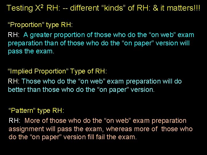
Testing X 2 RH: -- different “kinds” of RH: & it matters!!! “Proportion” type RH: A greater proportion of those who do the “on web” exam preparation than of those who do the “on paper” version will pass the exam. “Implied Proportion” Type of RH: Those who do the “on web” exam preparation will do better than those who do the “on paper” version. “Pattern” type RH: More of those who do the “on web” exam preparation assignment will pass the exam, whereas more of those who do the “on paper” version fill fail the exam.

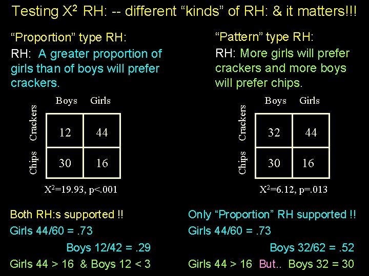
Testing X 2 RH: -- different “kinds” of RH: & it matters!!! Girls 12 44 30 16 X 2=19. 93, p<. 001 Both RH: s supported !! Girls 44/60 =. 73 Boys 12/42 =. 29 Girls 44 > 16 & Boys 12 < 3 Crackers Boys “Pattern” type RH: More girls will prefer crackers and more boys will prefer chips. Chips Crackers “Proportion” type RH: A greater proportion of girls than of boys will prefer crackers. Boys Girls 32 44 30 16 X 2=6. 12, p=. 013 Only “Proportion” RH supported !! Girls 44/60 =. 73 Boys 32/62 =. 52 Girls 44 > 16 But. . Boys 32 = 30

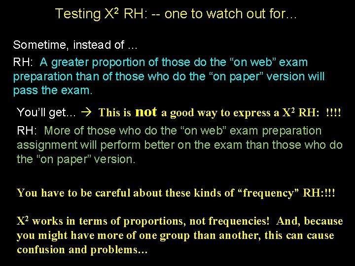
Testing X 2 RH: -- one to watch out for… Sometime, instead of … RH: A greater proportion of those do the “on web” exam preparation than of those who do the “on paper” version will pass the exam. You’ll get… This is not a good way to express a X 2 RH: !!!! RH: More of those who do the “on web” exam preparation assignment will perform better on the exam than those who do the “on paper” version. You have to be careful about these kinds of “frequency” RH: !!! X 2 works in terms of proportions, not frequencies! And, because you might have more of one group than another, this can cause confusion and problems…

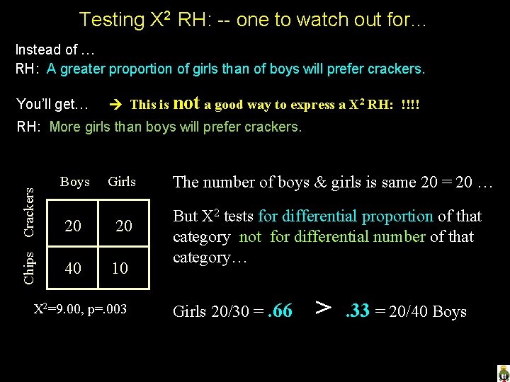
Testing X 2 RH: -- one to watch out for… Instead of … RH: A greater proportion of girls than of boys will prefer crackers. You’ll get… This is not a good way to express a X 2 RH: !!!! Chips Crackers RH: More girls than boys will prefer crackers. Boys Girls 20 20 40 10 X 2=9. 00, p=. 003 The number of boys & girls is same 20 = 20 … But X 2 tests for differential proportion of that category not for differential number of that category… Girls 20/30 =. 66 > . 33 = 20/40 Boys

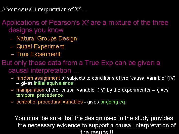
About causal interpretation of X². . . Applications of Pearson’s X² are a mixture of the three designs you know – Natural Groups Design – Quasi-Experiment – True Experiment But only those data from a True Exp can be given a causal interpretation … – random assignment of subjects to conditions of the “causal variable” (IV) -- gives initial equivalence. – manipulation of the “causal variable” (IV) by the experimenter -- gives temporal precedence – control of procedural variables - gives ongoing eq. You must be sure that the design used in the study provides the necessary evidence to support a causal interpretation of

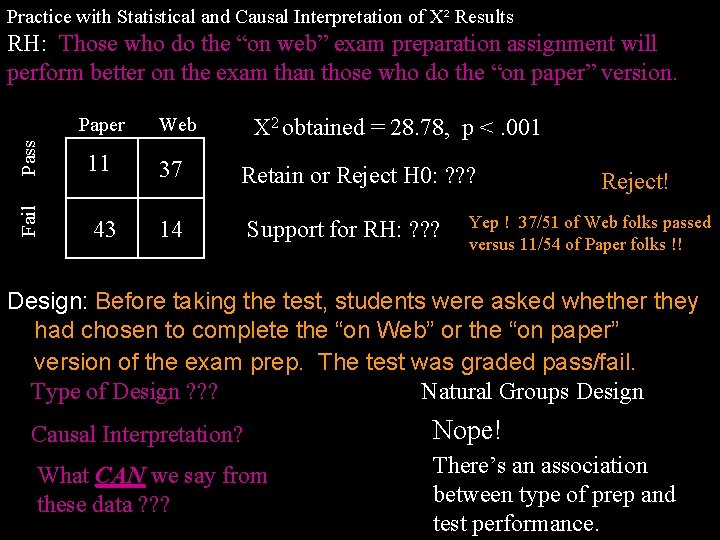
Practice with Statistical and Causal Interpretation of X² Results RH: Those who do the “on web” exam preparation assignment will perform better on the exam than those who do the “on paper” version. Web Pass X 2 obtained = 28. 78, p <. 001 11 37 Retain or Reject H 0: ? ? ? Fail Paper 43 14 Support for RH: ? ? ? Reject! Yep ! 37/51 of Web folks passed versus 11/54 of Paper folks !! Design: Before taking the test, students were asked whether they had chosen to complete the “on Web” or the “on paper” version of the exam prep. The test was graded pass/fail. Type of Design ? ? ? Natural Groups Design Causal Interpretation? Nope! What CAN we say from these data ? ? ? There’s an association between type of prep and test performance.

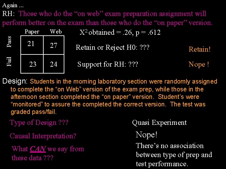
Again. . . Fail Pass RH: Those who do the “on web” exam preparation assignment will perform better on the exam than those who do the “on paper” version. Paper Web X 2 obtained =. 26, p =. 612 21 27 Retain or Reject H 0: ? ? ? Retain! 23 24 Support for RH: ? ? ? Nope ! Design: Students in the morning laboratory section were randomly assigned to complete the “on Web” version of the exam prep, while those in the afternoon section completed the “on paper” version. Student’s were “monitored” to assure the completed the correct version. The test was graded pass/fail. Type of Design ? ? ? Quasi Experiment Causal Interpretation? Nope! What CAN we say from these data ? ? ? There’s no association between type of prep and test performance.

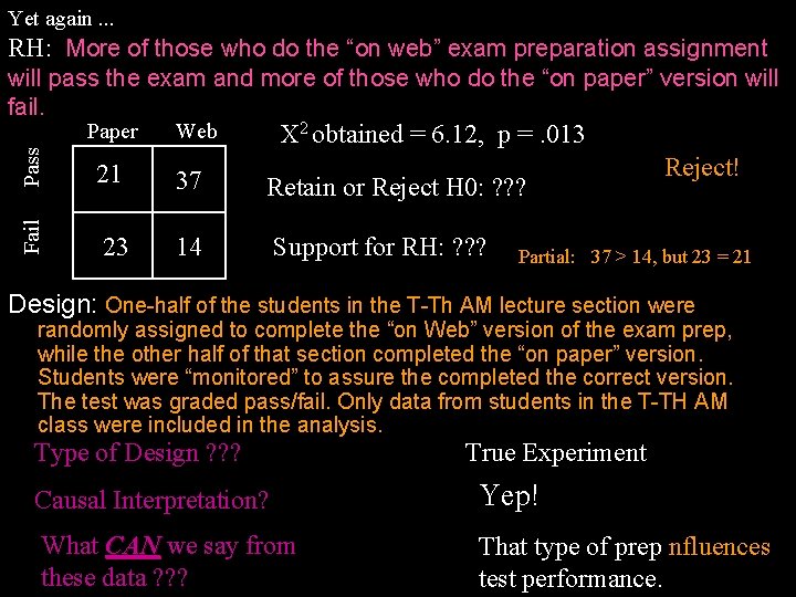
Yet again. . . RH: More of those who do the “on web” exam preparation assignment will pass the exam and more of those who do the “on paper” version will fail. Web Pass X 2 obtained = 6. 12, p =. 013 21 37 Retain or Reject H 0: ? ? ? Fail Paper 23 14 Support for RH: ? ? ? Reject! Partial: 37 > 14, but 23 = 21 Design: One-half of the students in the T-Th AM lecture section were randomly assigned to complete the “on Web” version of the exam prep, while the other half of that section completed the “on paper” version. Students were “monitored” to assure the completed the correct version. The test was graded pass/fail. Only data from students in the T-TH AM class were included in the analysis. Type of Design ? ? ? True Experiment Causal Interpretation? Yep! What CAN we say from these data ? ? ? That type of prep nfluences test performance.