Hypothesis Testing Null Hypothesis The means of the

Hypothesis Testing

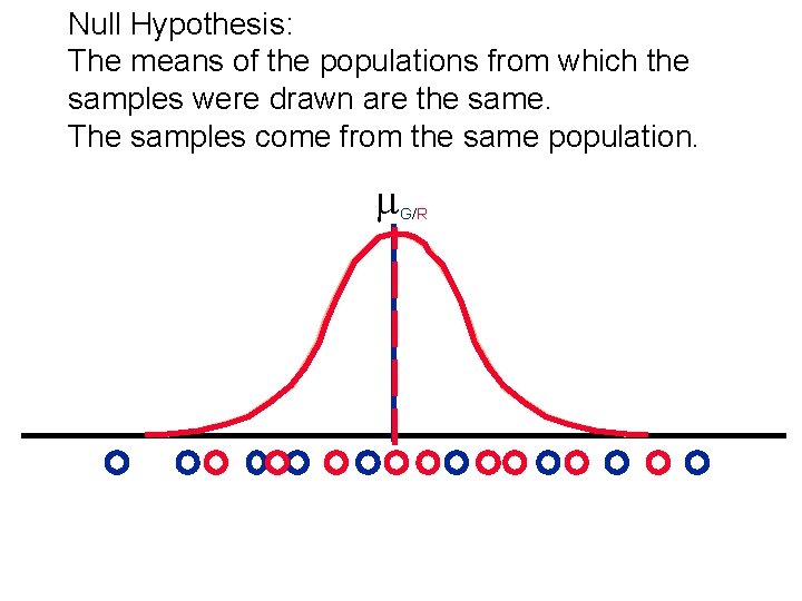
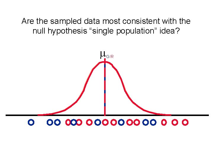
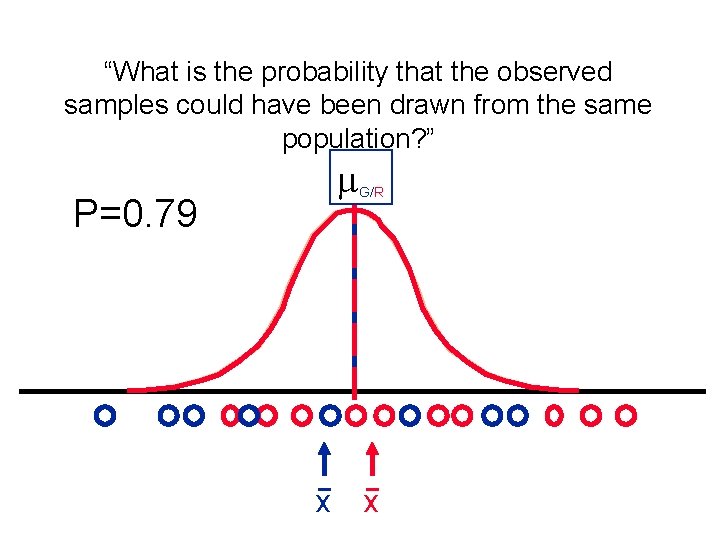
Null Hypothesis: The means of the populations from which the samples were drawn are the same. The samples come from the same population. m G/R

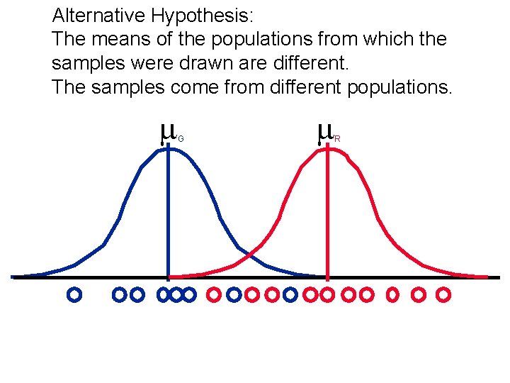
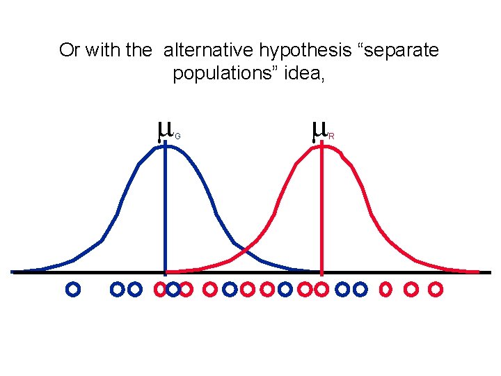
Alternative Hypothesis: The means of the populations from which the samples were drawn are different. The samples come from different populations. m G m R

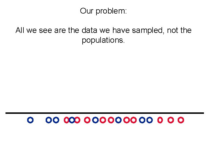
Our problem: All we see are the data we have sampled, not the populations.

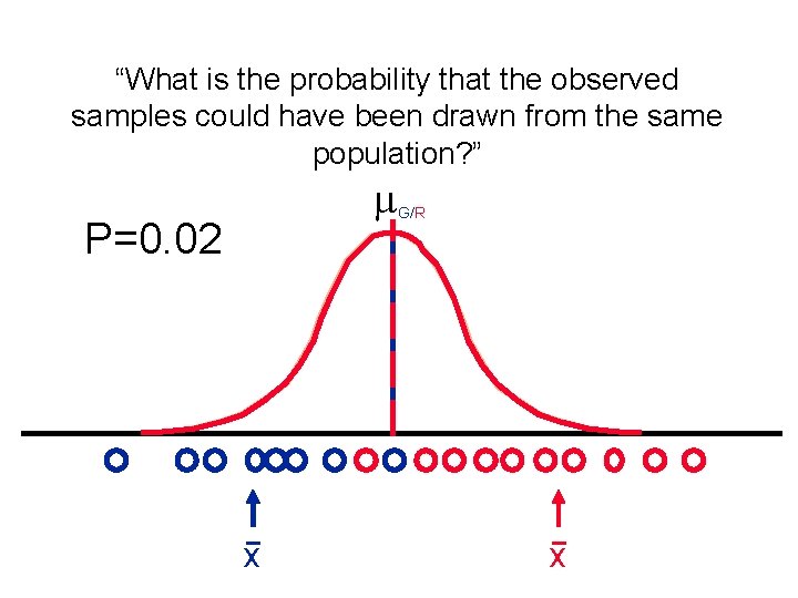
Are the sampled data most consistent with the null hypothesis “single population” idea? m G/R

Or with the alternative hypothesis “separate populations” idea, m G m R

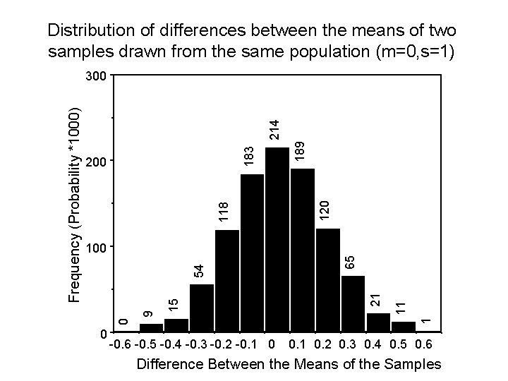
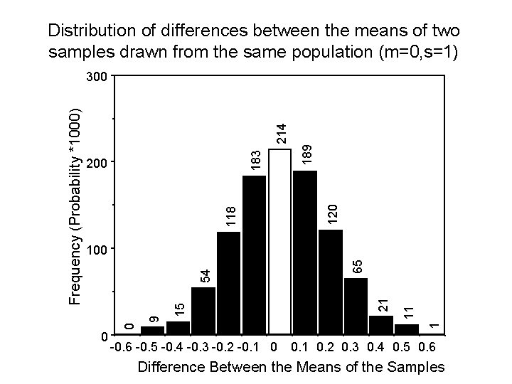
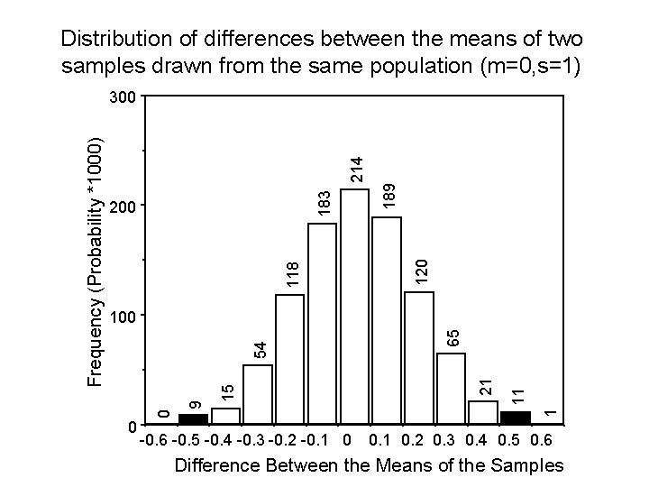
Distribution of differences between the means of two samples drawn from the same population (m=0, s=1) 0 -0. 6 -0. 5 -0. 4 -0. 3 -0. 2 -0. 1 0 1 11 65 120 21 15 9 54 100 189 214 183 118 200 0 Frequency (Probability *1000) 300 0. 1 0. 2 0. 3 0. 4 0. 5 0. 6 Difference Between the Means of the Samples

“What is the probability that the observed samples could have been drawn from the same population? ” m P=0. 79 x G/R x

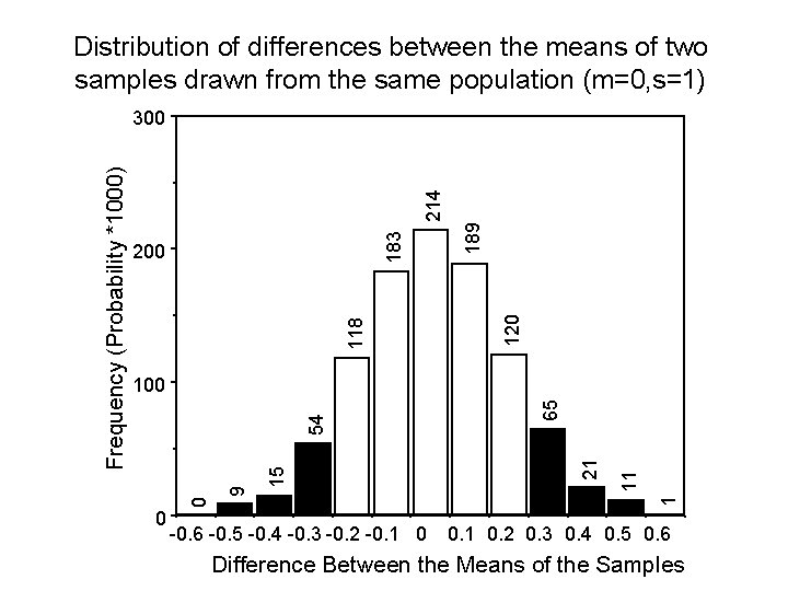
Distribution of differences between the means of two samples drawn from the same population (m=0, s=1) 120 189 214 183 118 200 0 -0. 6 -0. 5 -0. 4 -0. 3 -0. 2 -0. 1 0 1 11 65 21 15 9 54 100 0 Frequency (Probability *1000) 300 0. 1 0. 2 0. 3 0. 4 0. 5 0. 6 Difference Between the Means of the Samples

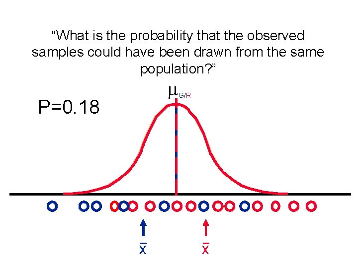
“What is the probability that the observed samples could have been drawn from the same population? ” m P=0. 18 x G/R x

Distribution of differences between the means of two samples drawn from the same population (m=0, s=1) 120 189 214 183 118 200 0 -0. 6 -0. 5 -0. 4 -0. 3 -0. 2 -0. 1 0 1 11 65 21 15 9 54 100 0 Frequency (Probability *1000) 300 0. 1 0. 2 0. 3 0. 4 0. 5 0. 6 Difference Between the Means of the Samples

“What is the probability that the observed samples could have been drawn from the same population? ” m P=0. 02 x G/R x

Distribution of differences between the means of two samples drawn from the same population (m=0, s=1) 120 189 214 183 118 200 0 -0. 6 -0. 5 -0. 4 -0. 3 -0. 2 -0. 1 0 1 11 65 21 15 9 54 100 0 Frequency (Probability *1000) 300 0. 1 0. 2 0. 3 0. 4 0. 5 0. 6 Difference Between the Means of the Samples

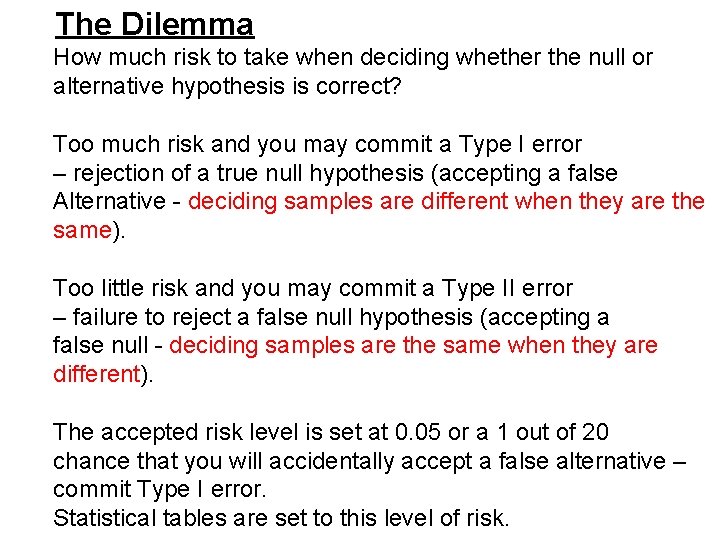
The Dilemma How much risk to take when deciding whether the null or alternative hypothesis is correct? Too much risk and you may commit a Type I error – rejection of a true null hypothesis (accepting a false Alternative - deciding samples are different when they are the same). Too little risk and you may commit a Type II error – failure to reject a false null hypothesis (accepting a false null - deciding samples are the same when they are different). The accepted risk level is set at 0. 05 or a 1 out of 20 chance that you will accidentally accept a false alternative – commit Type I error. Statistical tables are set to this level of risk.

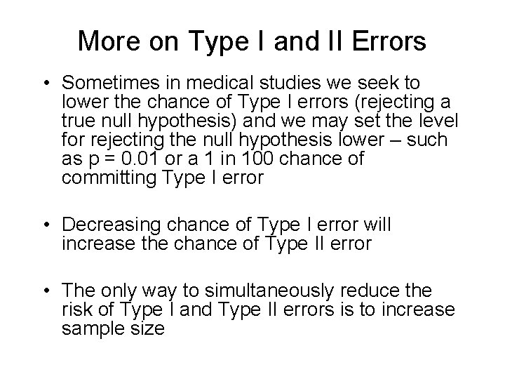
More on Type I and II Errors • Sometimes in medical studies we seek to lower the chance of Type I errors (rejecting a true null hypothesis) and we may set the level for rejecting the null hypothesis lower – such as p = 0. 01 or a 1 in 100 chance of committing Type I error • Decreasing chance of Type I error will increase the chance of Type II error • The only way to simultaneously reduce the risk of Type I and Type II errors is to increase sample size

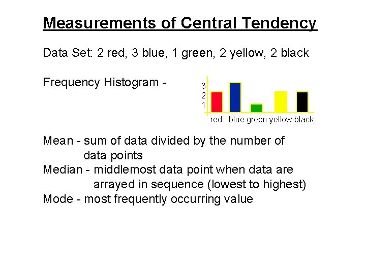
Measurements of Central Tendency Data Set: 2 red, 3 blue, 1 green, 2 yellow, 2 black Frequency Histogram - 3 2 1 red blue green yellow black Mean - sum of data divided by the number of data points Median - middlemost data point when data are arrayed in sequence (lowest to highest) Mode - most frequently occurring value

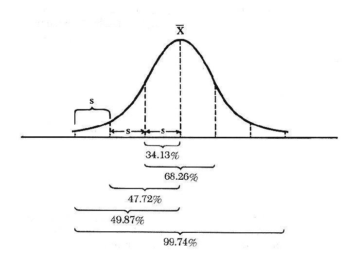
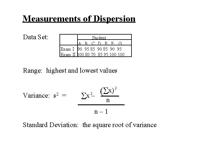
Measurements of Dispersion Data Set: Student A B C D E F G Exam I 90 95 85 90 95 Exam II 100 80 70 85 95 100 Range: highest and lowest values Variance: s 2 = 2 x) 2 x – n n– 1 Standard Deviation: the square root of variance