CONFIDENCE INTERVALS Confidence intervals for means and proportions

CONFIDENCE INTERVALS Confidence intervals for means and proportions: Section 6. 1 Section 7. 1 ( pages 450 – 453 ) Section 8. 1 ( pages 536 - 540 ) Topics: Point Estimates vs. Interval Estimates Context / Notation eight cases CI’s with z* assumptions interpretations tradeoffs choosing the right n CI’s with t* ( thanks to W. S. Gosset ) CI’s for proportions THE COOKBOOK

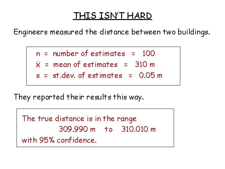
THIS ISN’T HARD Engineers measured the distance between two buildings. n = number of estimates = 100 x = mean of estimates = 310 m s = st. dev. of estimates = 0. 05 m They reported their results this way. The true distance is in the range 309. 990 m to 310. 010 m with 95% confidence.

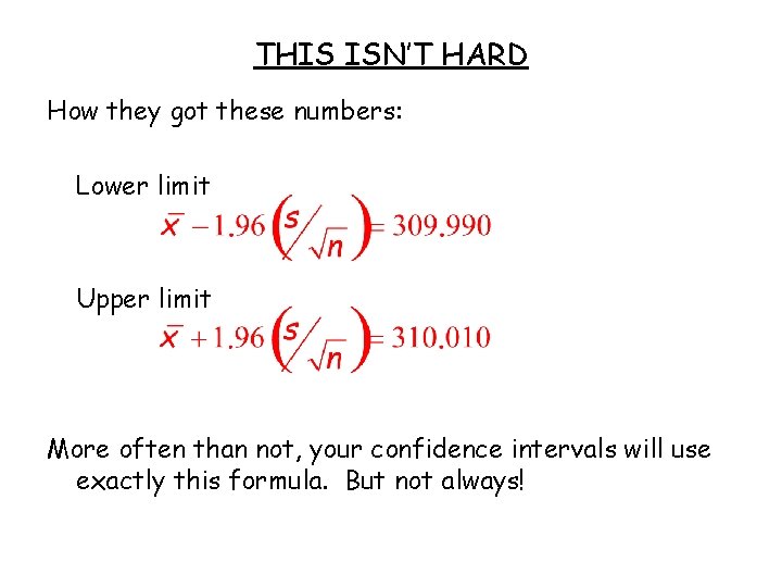
THIS ISN’T HARD How they got these numbers: Lower limit Upper limit More often than not, your confidence intervals will use exactly this formula. But not always!

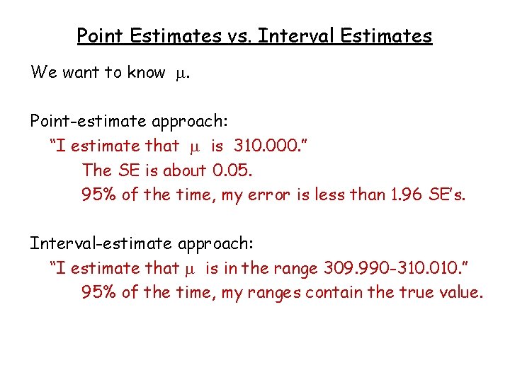
Point Estimates vs. Interval Estimates We want to know . Point-estimate approach: “I estimate that is 310. 000. ” The SE is about 0. 05. 95% of the time, my error is less than 1. 96 SE’s. Interval-estimate approach: “I estimate that is in the range 309. 990 -310. 010. ” 95% of the time, my ranges contain the true value.

Interval estimates Two things you want to know about an interval estimate: (a) the interval, of course (b) the CONFIDENCE LEVEL, or CONTAINMENT PROBABILITY. What fraction of intervals constructed in this way contain the true value?

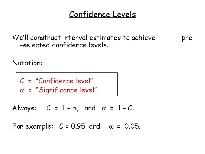
Confidence Levels We’ll construct interval estimates to achieve -selected confidence levels. Notation: C = “Confidence level” = “Significance level” Always: C = 1 - , and = 1 – C. For example: C = 0. 95 and = 0. 05. pre

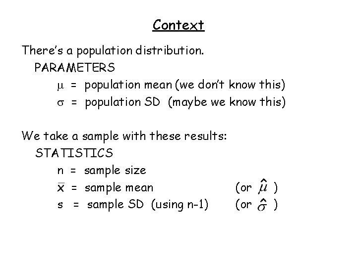
Context There’s a population distribution. PARAMETERS = population mean (we don’t know this) = population SD (maybe we know this) We take a sample with these results: STATISTICS n = sample size x = sample mean (or s = sample SD (using n-1) (or ) )

At least 8 cases n large vs. n small known vs. unknown population roughly normal vs. non-normal or unknown (and we’ll consider proportions, too)

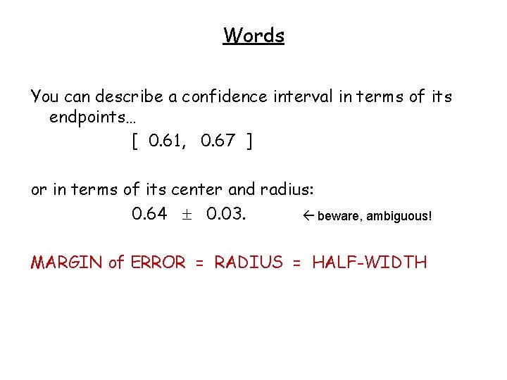
Words You can describe a confidence interval in terms of its endpoints… [ 0. 61, 0. 67 ] or in terms of its center and radius: 0. 64 0. 03. beware, ambiguous! MARGIN of ERROR = RADIUS = HALF-WIDTH

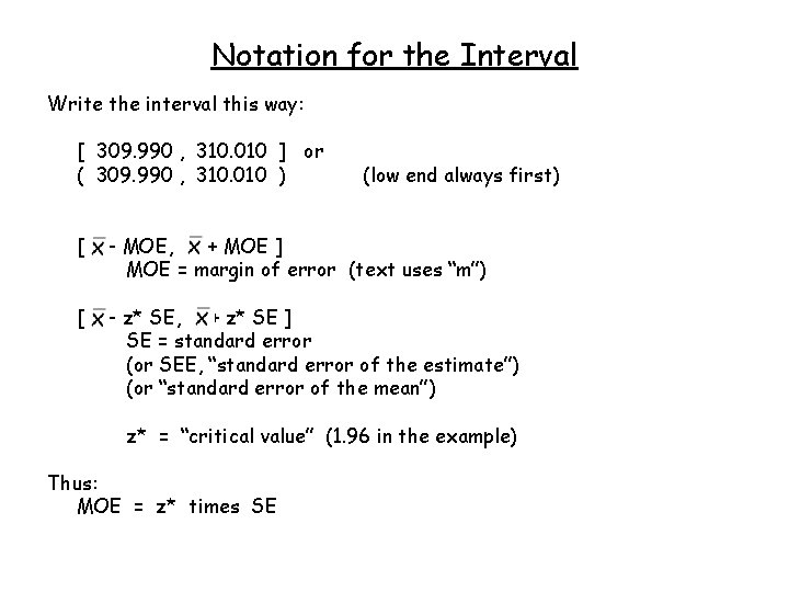
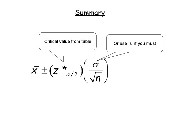
Notation for the Interval Write the interval this way: [ 309. 990 , 310. 010 ] or ( 309. 990 , 310. 010 ) (low end always first) [ x – MOE, x + MOE ] MOE = margin of error (text uses “m”) [ x – z* SE, x + z* SE ] SE = standard error (or SEE, “standard error of the estimate”) (or “standard error of the mean”) z* = “critical value” (1. 96 in the example) Thus: MOE = z* times SE

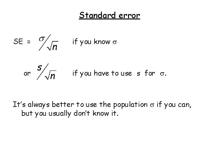
Standard error SE = or if you know if you have to use s for . It’s always better to use the population if you can, but you usually don’t know it.

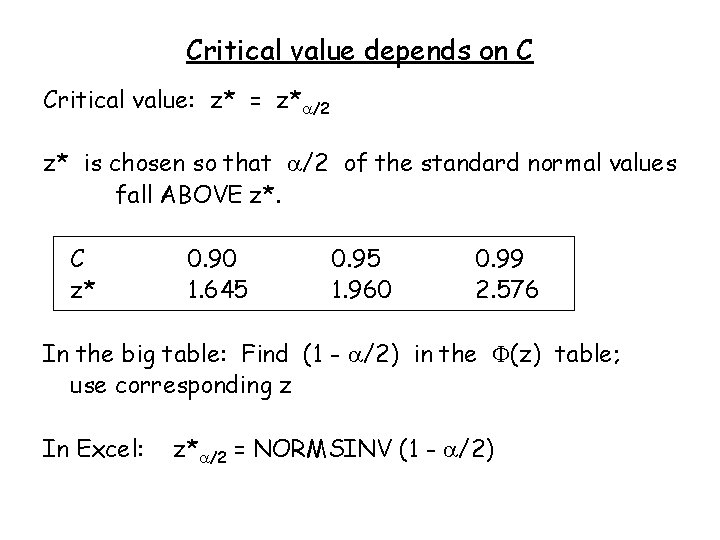
Critical value depends on C Critical value: z* = z* /2 z* is chosen so that /2 of the standard normal values fall ABOVE z*. C z* 0. 90 1. 645 0. 95 1. 960 0. 99 2. 576 In the big table: Find (1 - /2) in the (z) table; use corresponding z In Excel: z* /2 = NORMSINV (1 - /2)

Summary Critical value from table Or use s if you must

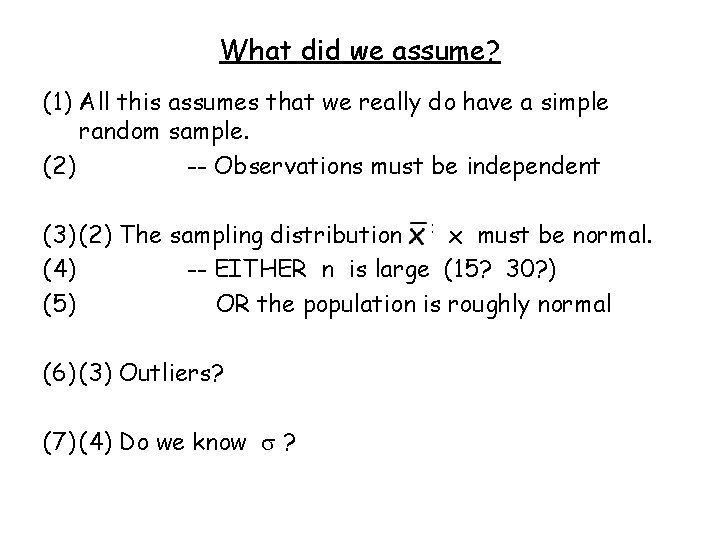
What did we assume? (1) All this assumes that we really do have a simple random sample. (2) -- Observations must be independent (3) (2) The sampling distribution of x must be normal. (4) -- EITHER n is large (15? 30? ) (5) OR the population is roughly normal (6) (3) Outliers? (7) (4) Do we know ?

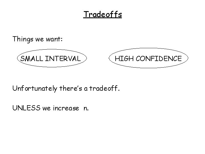
Tradeoffs Things we want: SMALL INTERVAL HIGH CONFIDENCE Unfortunately there’s a tradeoff. UNLESS we increase n.

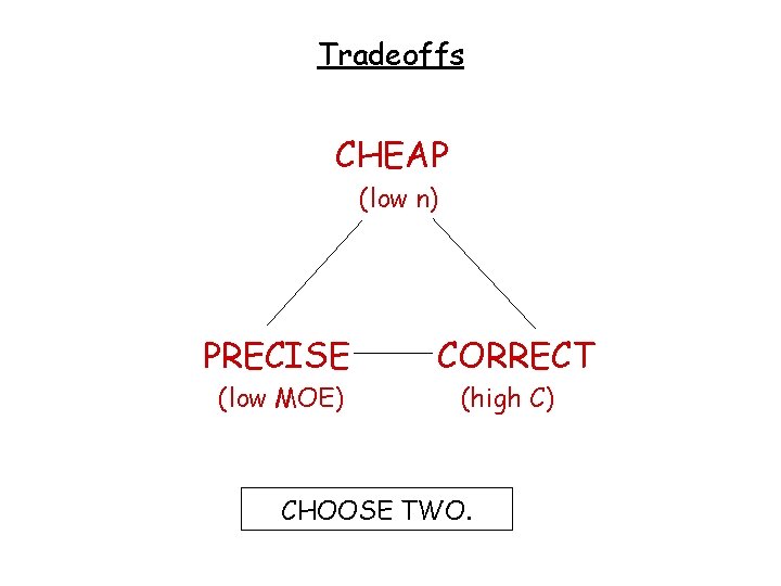
Tradeoffs CHEAP (low n) PRECISE (low MOE) CORRECT (high C) CHOOSE TWO.

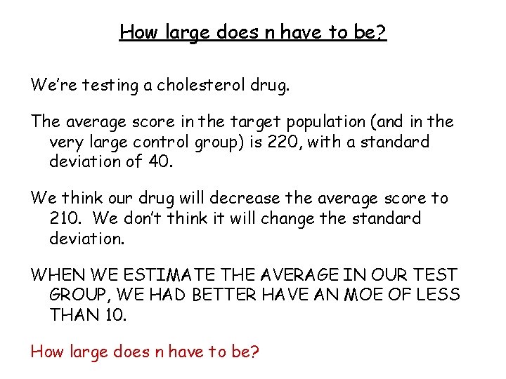
How large does n have to be? We’re testing a cholesterol drug. The average score in the target population (and in the very large control group) is 220, with a standard deviation of 40. We think our drug will decrease the average score to 210. We don’t think it will change the standard deviation. WHEN WE ESTIMATE THE AVERAGE IN OUR TEST GROUP, WE HAD BETTER HAVE AN MOE OF LESS THAN 10. How large does n have to be?

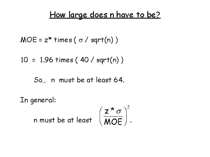
How large does n have to be? MOE = z* times ( / sqrt(n) ) 10 = 1. 96 times ( 40 / sqrt(n) ) So… n must be at least 64. In general: n must be at least .

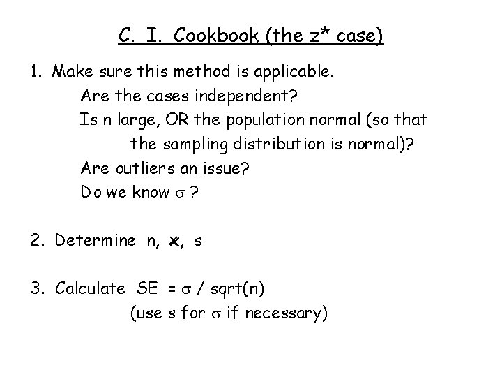
C. I. Cookbook (the z* case) 1. Make sure this method is applicable. Are the cases independent? Is n large, OR the population normal (so that the sampling distribution is normal)? Are outliers an issue? Do we know ? 2. Determine n, x, s 3. Calculate SE = / sqrt(n) (use s for if necessary)

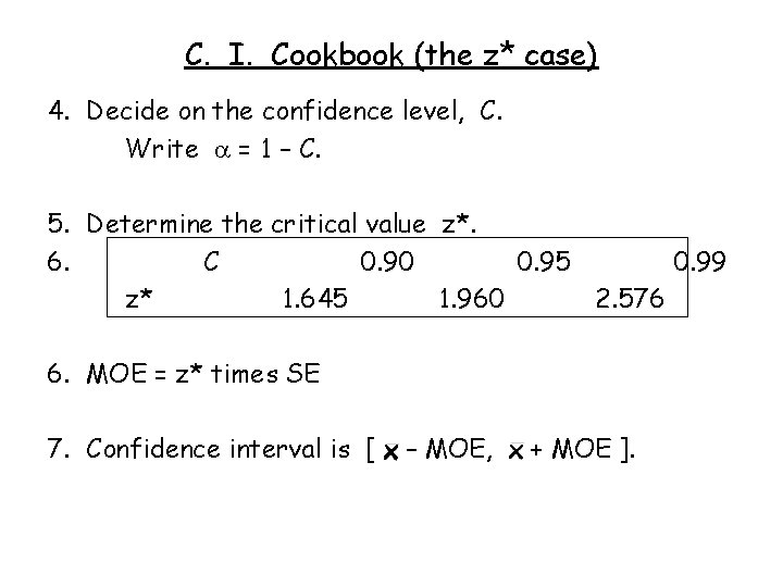
C. I. Cookbook (the z* case) 4. Decide on the confidence level, C. Write = 1 – C. 5. Determine the critical value z*. 6. C 0. 90 0. 95 0. 99 z* 1. 645 1. 960 2. 576 6. MOE = z* times SE 7. Confidence interval is [ x – MOE, x + MOE ].

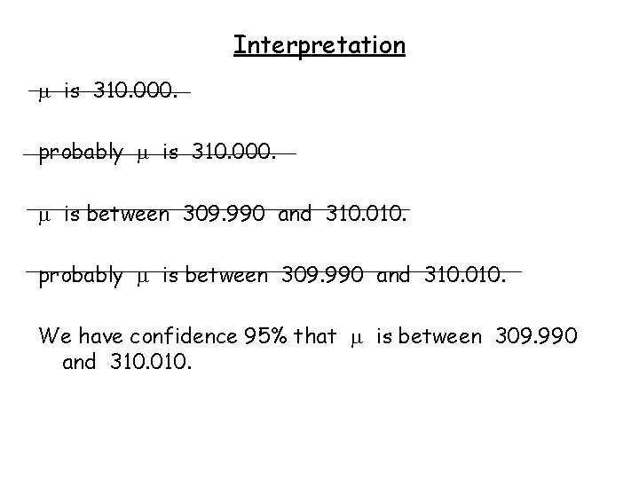
Interpretation is 310. 000.

Interpretation is 310. 000. probably is 310. 000.

Interpretation is 310. 000. probably is 310. 000. is between 309. 990 and 310. 010.

Interpretation is 310. 000. probably is 310. 000. is between 309. 990 and 310. 010. probably is between 309. 990 and 310. 010.

Interpretation is 310. 000. probably is 310. 000. is between 309. 990 and 310. 010. probably is between 309. 990 and 310. 010. We have confidence 95% that is between 309. 990 and 310. 010.

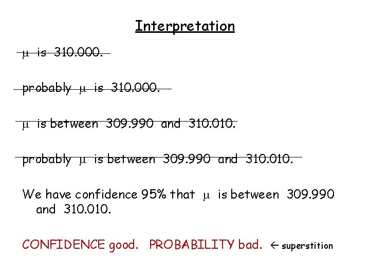
Interpretation is 310. 000. probably is 310. 000. is between 309. 990 and 310. 010. probably is between 309. 990 and 310. 010. We have confidence 95% that is between 309. 990 and 310. 010. CONFIDENCE good. PROBABILITY bad. superstition

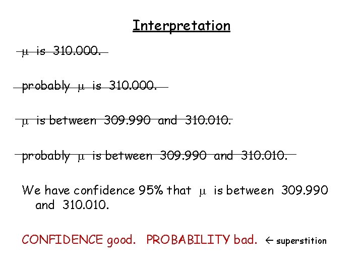
Interpretation is 310. 000. probably is 310. 000. is between 309. 990 and 310. 010. probably is between 309. 990 and 310. 010. We have confidence 95% that is between 309. 990 and 310. 010. CONFIDENCE good. PROBABILITY bad. superstition

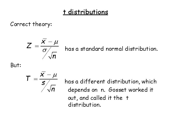
t distributions Everything we have done so far assumes that the sampling distribution is normal. W. S. Gosset made the same assumption at the Guinness Brewing Company, but he kept getting bad results. His population distribution was roughly normal, but his sample sizes were small. And, like most people, he had to use s for .

W. S. Gosset “A. Student”

t distributions Correct theory: has a standard normal distribution. But: has a different distribution, which depends on n. Gosset worked it out, and called it the t distribution.

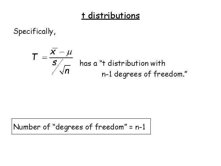
t distributions Specifically, has a “t distribution with n-1 degrees of freedom. ” Number of “degrees of freedom” = n-1

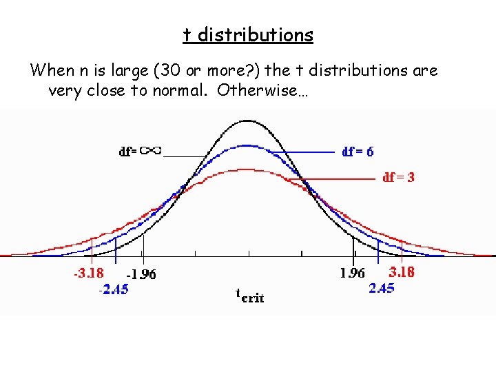
t distributions When n is large (30 or more? ) the t distributions are very close to normal. Otherwise…

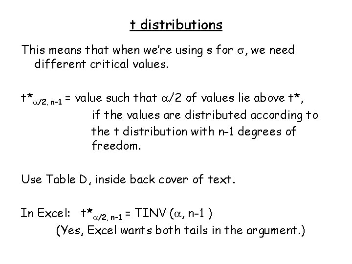
t distributions This means that when we’re using s for , we need different critical values. t* /2, n-1 = value such that /2 of values lie above t*, if the values are distributed according to the t distribution with n-1 degrees of freedom. Use Table D, inside back cover of text. In Excel: t* /2, n-1 = TINV ( , n-1 ) (Yes, Excel wants both tails in the argument. )

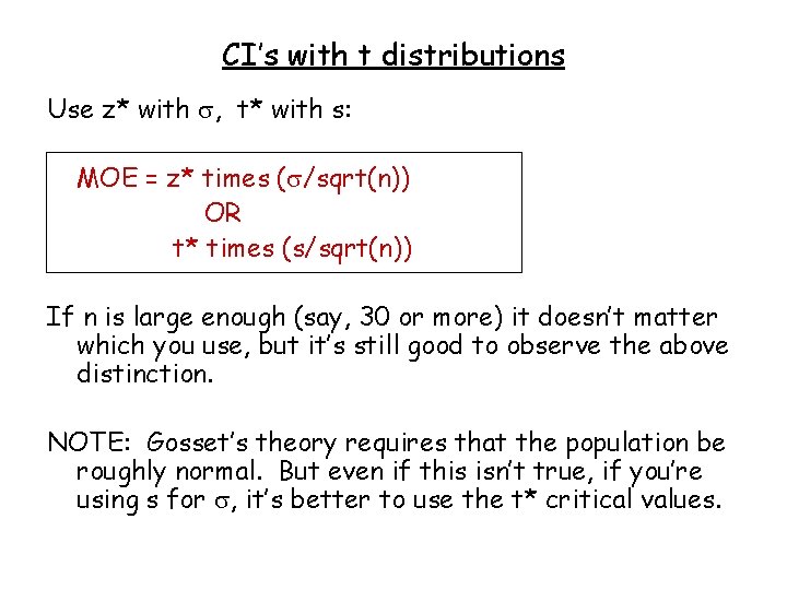
CI’s with t distributions Use z* with , t* with s: MOE = z* times ( /sqrt(n)) OR t* times (s/sqrt(n)) If n is large enough (say, 30 or more) it doesn’t matter which you use, but it’s still good to observe the above distinction. NOTE: Gosset’s theory requires that the population be roughly normal. But even if this isn’t true, if you’re using s for , it’s better to use the t* critical values.

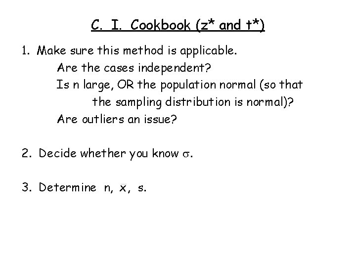
C. I. Cookbook (z* and t*) 1. Make sure this method is applicable. Are the cases independent? Is n large, OR the population normal (so that the sampling distribution is normal)? Are outliers an issue? 2. Decide whether you know . 3. Determine n, x, s.

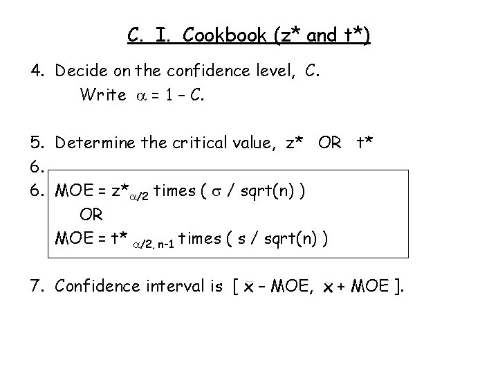
C. I. Cookbook (z* and t*) 4. Decide on the confidence level, C. Write = 1 – C. 5. Determine the critical value, z* OR t* 6. 6. MOE = z* /2 times ( / sqrt(n) ) OR MOE = t* /2, n-1 times ( s / sqrt(n) ) 7. Confidence interval is [ x – MOE, x + MOE ].

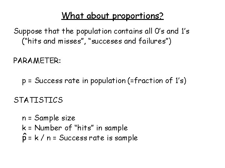
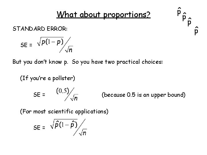
What about proportions? Suppose that the population contains all 0’s and 1’s (“hits and misses”, “succeses and failures”) PARAMETER: p = Success rate in population (=fraction of 1’s) STATISTICS n = Sample size k = Number of “hits” in sample p = k / n = Success rate is sample

What about proportions? STANDARD ERROR: SE = But you don’t know p. So you have two practical choices: (If you’re a pollster) SE = (because 0. 5 is an upper bound) (For most scientific applications) SE =

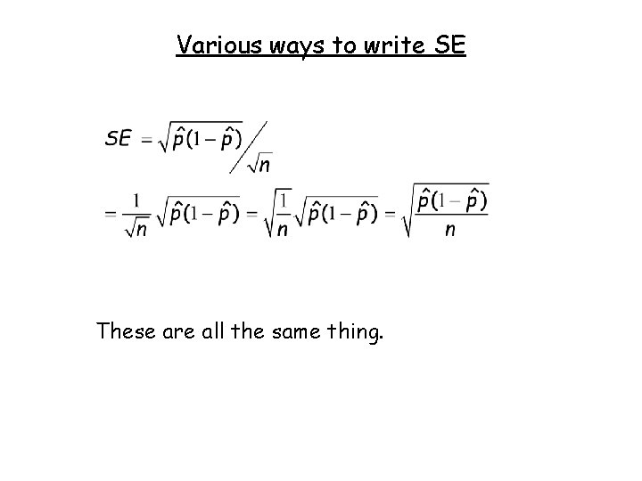
Various ways to write SE These are all the same thing.

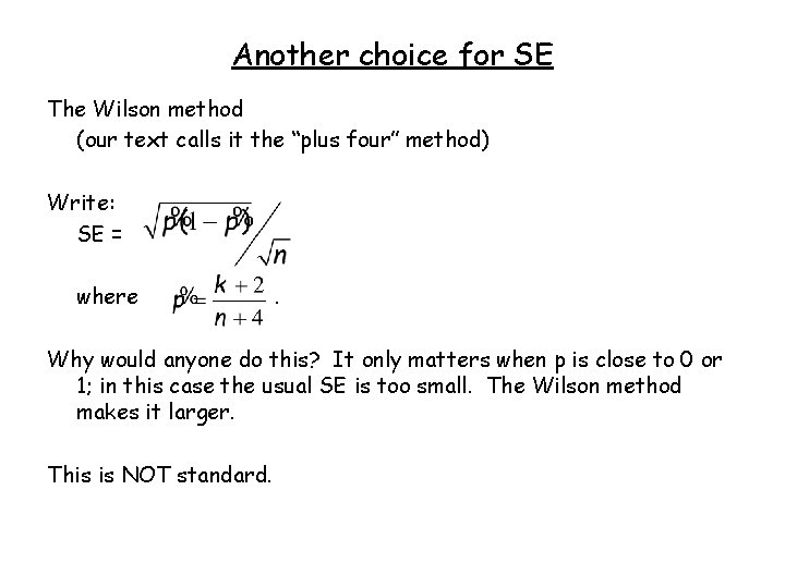
Another choice for SE The Wilson method (our text calls it the “plus four” method) Write: SE = where . Why would anyone do this? It only matters when p is close to 0 or 1; in this case the usual SE is too small. The Wilson method makes it larger. This is NOT standard.

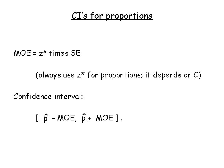
CI’s for proportions MOE = z* times SE (always use z* for proportions; it depends on C) Confidence interval: [ - MOE, + MOE ].

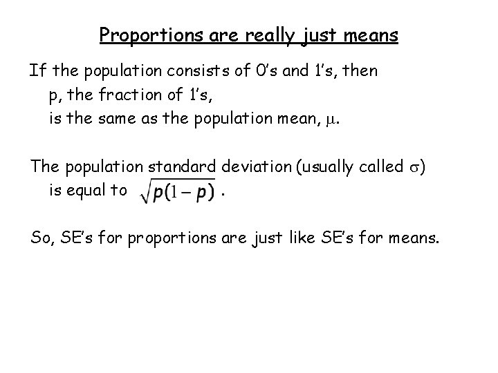
Proportions are really just means If the population consists of 0’s and 1’s, then p, the fraction of 1’s, is the same as the population mean, . The population standard deviation (usually called ) is equal to. So, SE’s for proportions are just like SE’s for means.

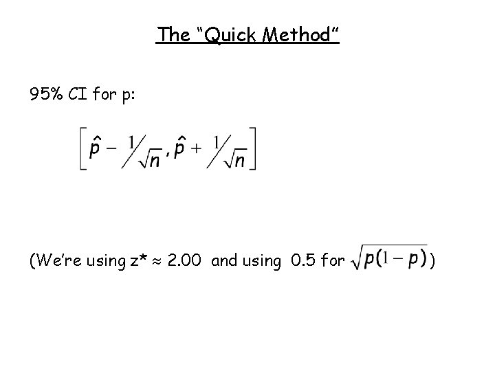
The “Quick Method” 95% CI for p: (We’re using z* 2. 00 and using 0. 5 for )

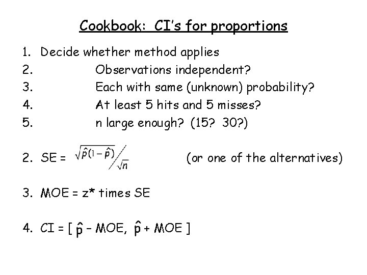
Cookbook: CI’s for proportions 1. Decide whether method applies 2. Observations independent? 3. Each with same (unknown) probability? 4. At least 5 hits and 5 misses? 5. n large enough? (15? 30? ) 2. SE = (or one of the alternatives) 3. MOE = z* times SE 4. CI = [ p – MOE, p + MOE ]