Interval Estimation 2 Computing Confidence Intervals Confidence Intervals

Interval Estimation 2 Computing Confidence Intervals

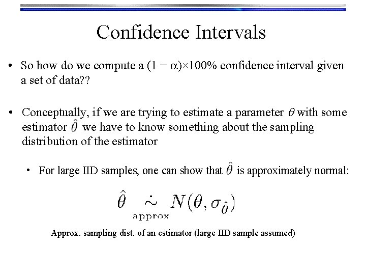
Confidence Intervals • So how do we compute a (1 − a)× 100% confidence interval given a set of data? ? • Conceptually, if we are trying to estimate a parameter q with some estimator we have to know something about the sampling distribution of the estimator • For large IID samples, one can show that is approximately normal: Approx. sampling dist. of an estimator (large IID sample assumed)

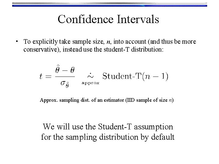
Confidence Intervals • To explicitly take sample size, n, into account (and thus be more conservative), instead use the student-T distribution: Approx. sampling dist. of an estimator (IID sample of size n) We will use the Student-T assumption for the sampling distribution by default

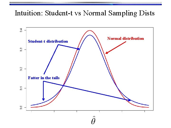
Intuition: Student-t vs Normal Sampling Dists Student-t distribution Fatter in the tails Normal distribution

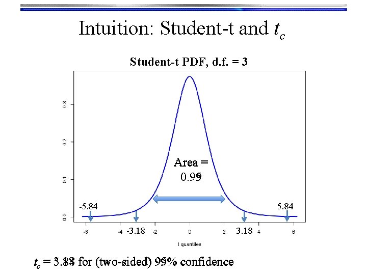
Intuition: Student-t and tc Student-t PDF, d. f. = 3 Area = 0. 99 0. 95 5. 84 -3. 18 for (two-sided) 99% 95% confidence tc = 5. 84 3. 18

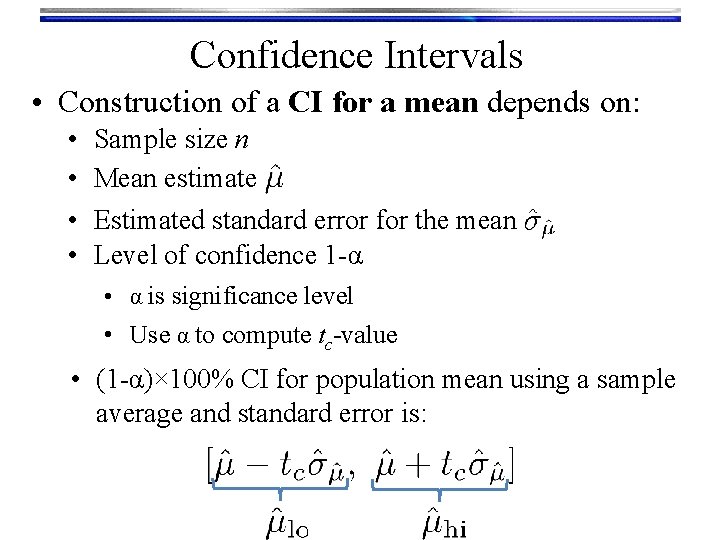
Confidence Intervals • Construction of a CI for a mean depends on: • • Sample size n Mean estimate Estimated standard error for the mean Level of confidence 1 -α • α is significance level • Use α to compute tc-value • (1 -α)× 100% CI for population mean using a sample average and standard error is:

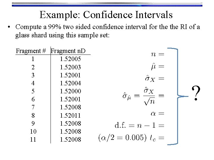
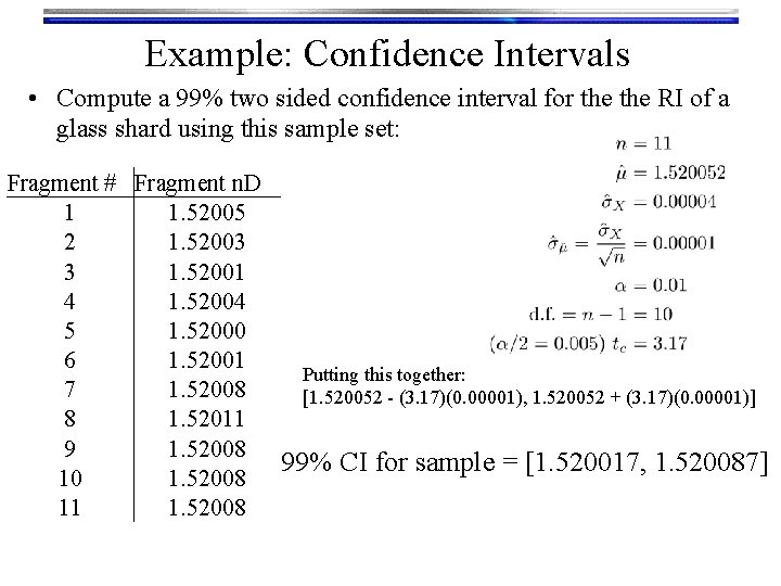
Example: Confidence Intervals • Compute a 99% two sided confidence interval for the RI of a glass shard using this sample set: Fragment # Fragment n. D 1 1. 52005 2 1. 52003 3 1. 52001 4 1. 52004 5 1. 52000 6 1. 52001 7 1. 52008 8 1. 52011 9 1. 52008 10 1. 52008 11 1. 52008 ?

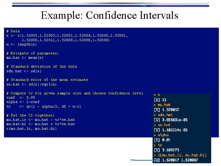
Example: Confidence Intervals # Data x <- c(1. 52005, 1. 52003, 1. 52001, 1. 52004, 1. 52000, 1. 52001, 1. 52008, 1. 52011, 1. 52008, 1. 52008) n <- length(x) # Estimate of parameter: mu. hat <- mean(x) # Standard deviation of the data sdx. hat <- sd(x) # Standard error of the mean estimate se. hat <- sd(x)/sqrt(n) # Compute tc for given sample size and chosen confidence level conf <- 0. 99 alpha <- 1 -conf tc <- qt(1 - alpha/2, df = n-1) # Put the CI mu. hat. lo <mu. hat. hi <c(mu. hat. lo, together: mu. hat - tc*se. hat mu. hat + tc*se. hat mu. hat. hi)

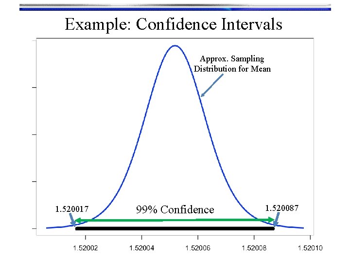
Example: Confidence Intervals Approx. Sampling Distribution for Mean 1. 520017 99% Confidence 1. 520087

Example: Confidence Intervals • Compute a 99% two sided confidence interval for the RI of a glass shard using this sample set: Fragment # Fragment n. D 1 1. 52005 2 1. 52003 3 1. 52001 4 1. 52004 5 1. 52000 6 1. 52001 Putting this together: 7 1. 52008 [1. 520052 - (3. 17)(0. 00001), 1. 520052 + (3. 17)(0. 00001)] 8 1. 52011 9 1. 52008 99% CI for sample = [1. 520017, 1. 520087] 10 1. 52008 11 1. 52008

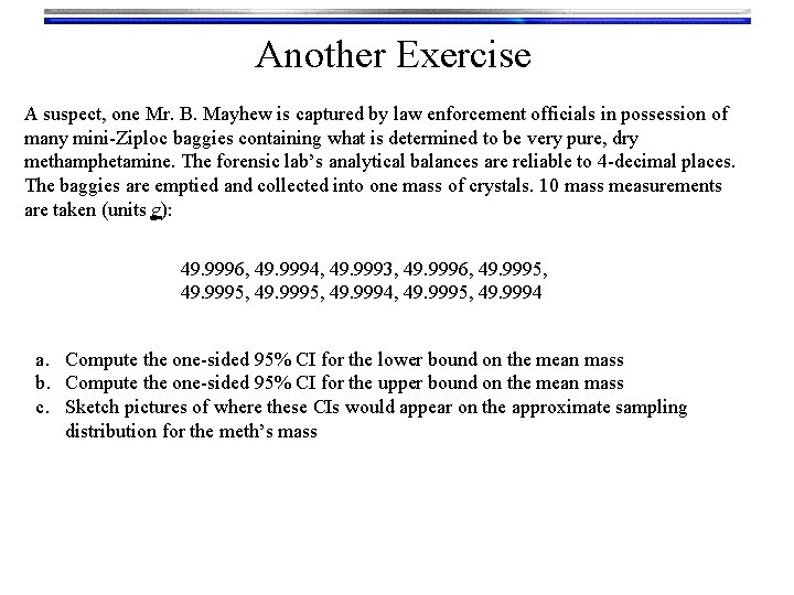
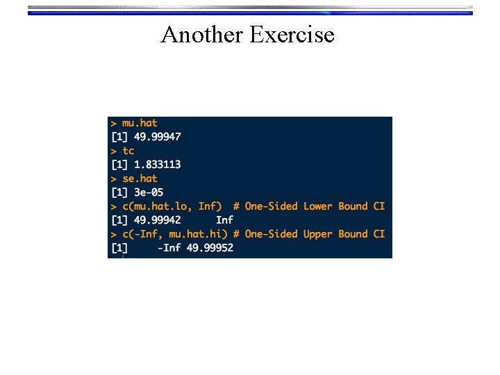
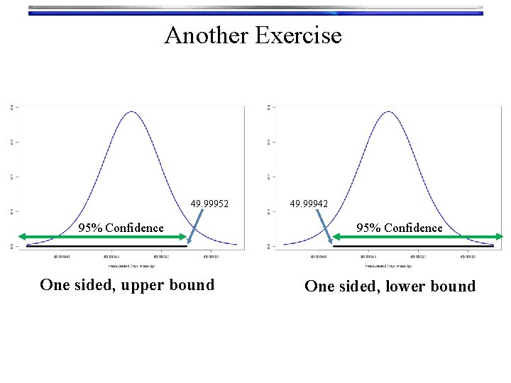
Another Exercise A suspect, one Mr. B. Mayhew is captured by law enforcement officials in possession of many mini-Ziploc baggies containing what is determined to be very pure, dry methamphetamine. The forensic lab’s analytical balances are reliable to 4 -decimal places. The baggies are emptied and collected into one mass of crystals. 10 mass measurements are taken (units g): 49. 9996, 49. 9994, 49. 9993, 49. 9996, 49. 9995, 49. 9994 a. Compute the one-sided 95% CI for the lower bound on the mean mass b. Compute the one-sided 95% CI for the upper bound on the mean mass c. Sketch pictures of where these CIs would appear on the approximate sampling distribution for the meth’s mass

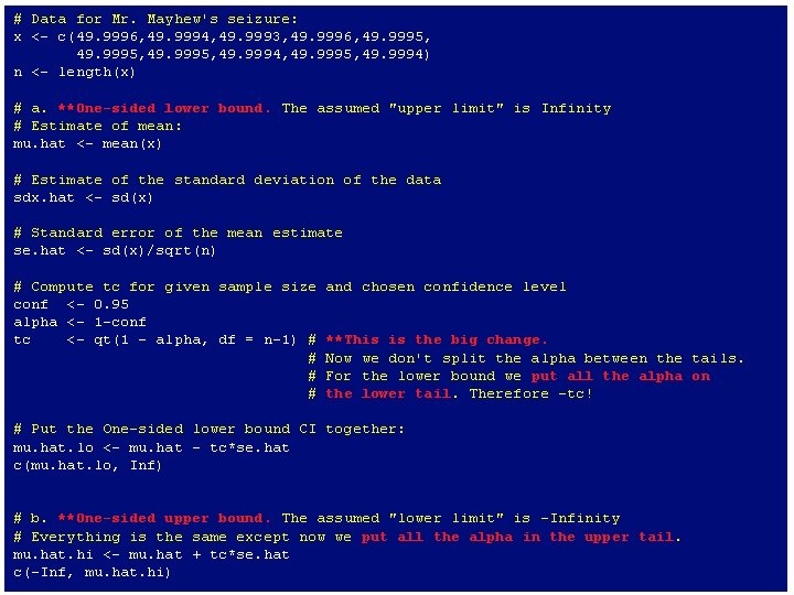
# Data for Mr. Mayhew's seizure: x <- c(49. 9996, 49. 9994, 49. 9993, 49. 9996, 49. 9995, 49. 9994) n <- length(x) # a. **One-sided lower bound. The assumed "upper limit" is Infinity # Estimate of mean: mu. hat <- mean(x) # Estimate of the standard deviation of the data sdx. hat <- sd(x) # Standard error of the mean estimate se. hat <- sd(x)/sqrt(n) # Compute tc for given sample size conf <- 0. 95 alpha <- 1 -conf tc <- qt(1 - alpha, df = n-1) # # and chosen confidence level **This is the big change. Now we don't split the alpha between the tails. For the lower bound we put all the alpha on the lower tail. Therefore -tc! # Put the One-sided lower bound CI together: mu. hat. lo <- mu. hat - tc*se. hat c(mu. hat. lo, Inf) # b. **One-sided upper bound. The assumed "lower limit" is -Infinity # Everything is the same except now we put all the alpha in the upper tail. mu. hat. hi <- mu. hat + tc*se. hat c(-Inf, mu. hat. hi)

Another Exercise

Another Exercise 49. 99952 95% Confidence One sided, upper bound 49. 99942 95% Confidence One sided, lower bound