Confidence Intervals and Upper Limits Confidence intervals CI

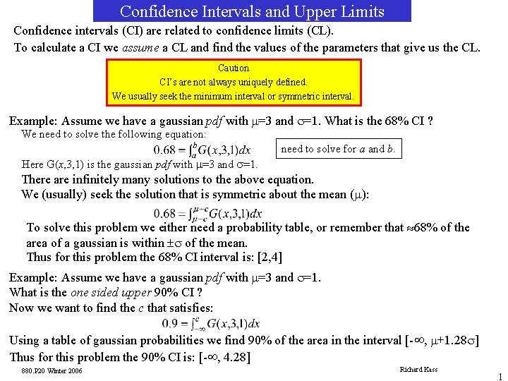
Confidence Intervals and Upper Limits Confidence intervals (CI) are related to confidence limits (CL). To calculate a CI we assume a CL and find the values of the parameters that give us the CL. Caution CI’s are not always uniquely defined. We usually seek the minimum interval or symmetric interval. Example: Assume we have a gaussian pdf with m=3 and s=1. What is the 68% CI ? We need to solve the following equation: need to solve for a and b. Here G(x, 3, 1) is the gaussian pdf with m=3 and s=1. There are infinitely many solutions to the above equation. We (usually) seek the solution that is symmetric about the mean (m): To solve this problem we either need a probability table, or remember that » 68% of the area of a gaussian is within ±s of the mean. Thus for this problem the 68% CI interval is: [2, 4] Example: Assume we have a gaussian pdf with m=3 and s=1. What is the one sided upper 90% CI ? Now we want to find the c that satisfies: Using a table of gaussian probabilities we find 90% of the area in the interval [-¥, m+1. 28 s] Thus for this problem the 90% CI is: [-¥, 4. 28] 880. P 20 Winter 2006 Richard Kass 1

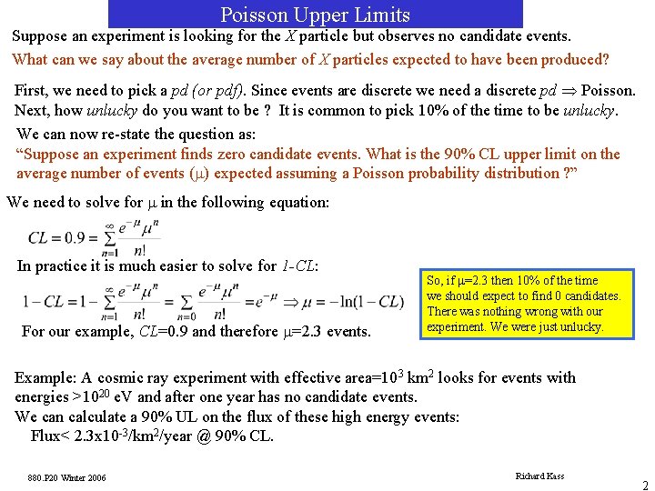
Poisson Upper Limits Suppose an experiment is looking for the X particle but observes no candidate events. What can we say about the average number of X particles expected to have been produced? First, we need to pick a pd (or pdf). Since events are discrete we need a discrete pd Þ Poisson. Next, how unlucky do you want to be ? It is common to pick 10% of the time to be unlucky. We can now re-state the question as: “Suppose an experiment finds zero candidate events. What is the 90% CL upper limit on the average number of events (m) expected assuming a Poisson probability distribution ? ” We need to solve for m in the following equation: In practice it is much easier to solve for 1 -CL: For our example, CL=0. 9 and therefore m=2. 3 events. So, if m=2. 3 then 10% of the time we should expect to find 0 candidates. There was nothing wrong with our experiment. We were just unlucky. Example: A cosmic ray experiment with effective area=103 km 2 looks for events with energies >1020 e. V and after one year has no candidate events. We can calculate a 90% UL on the flux of these high energy events: Flux< 2. 3 x 10 -3/km 2/year @ 90% CL. 880. P 20 Winter 2006 Richard Kass 2

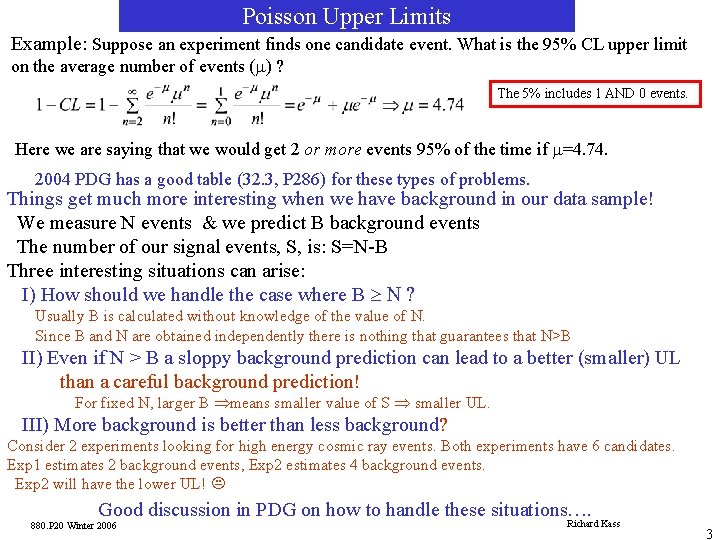
Poisson Upper Limits Example: Suppose an experiment finds one candidate event. What is the 95% CL upper limit on the average number of events (m) ? The 5% includes 1 AND 0 events. Here we are saying that we would get 2 or more events 95% of the time if m=4. 74. 2004 PDG has a good table (32. 3, P 286) for these types of problems. Things get much more interesting when we have background in our data sample! We measure N events & we predict B background events The number of our signal events, S, is: S=N-B Three interesting situations can arise: I) How should we handle the case where B ³ N ? Usually B is calculated without knowledge of the value of N. Since B and N are obtained independently there is nothing that guarantees that N>B II) Even if N > B a sloppy background prediction can lead to a better (smaller) UL than a careful background prediction! For fixed N, larger B Þmeans smaller value of S Þ smaller UL. III) More background is better than less background? Consider 2 experiments looking for high energy cosmic ray events. Both experiments have 6 candidates. Exp 1 estimates 2 background events, Exp 2 estimates 4 background events. Exp 2 will have the lower UL! K Good discussion in PDG on how to handle these situations…. 880. P 20 Winter 2006 Richard Kass 3

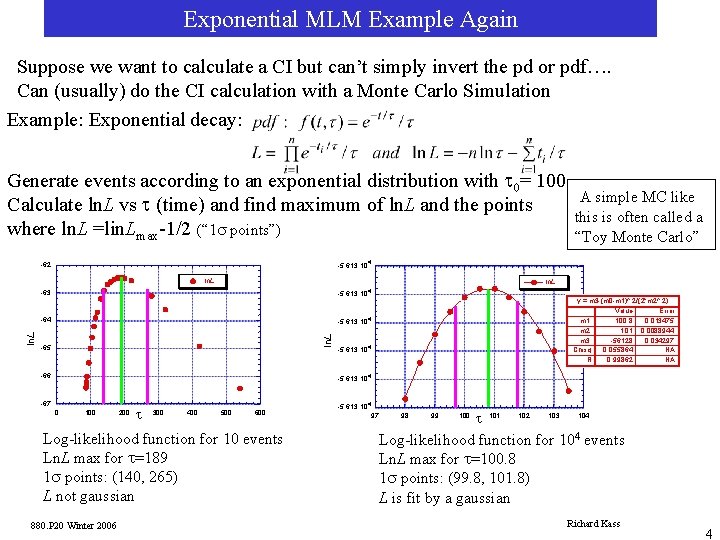
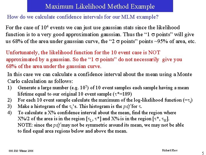
Exponential MLM Example Again Suppose we want to calculate a CI but can’t simply invert the pd or pdf…. Can (usually) do the CI calculation with a Monte Carlo Simulation Example: Exponential decay: Generate events according to an exponential distribution with t 0= 100 Calculate ln. L vs t (time) and find maximum of ln. L and the points where ln. L =lin. Lmax-1/2 (“ 1 s points”) -5. 613 10 4 -62 ln. L -5. 613 10 4 -63 -64 y = m 3 -(m 0 -m 1)^ 2/(2*m 2^ 2) Value Error m 1 100. 8 0. 013475 m 2 1. 01 0. 0088944 m 3 -56128 0. 034297 Chisq 0. 055864 NA R 0. 99862 NA -5. 613 10 4 ln. L A simple MC like this is often called a “Toy Monte Carlo” -65 -66 -5. 613 10 4 -67 0 100 200 t 300 400 500 600 Log-likelihood function for 10 events Ln. L max for t=189 1 s points: (140, 265) L not gaussian 880. P 20 Winter 2006 -5. 613 10 4 97 98 99 100 t 101 102 103 104 Log-likelihood function for 104 events Ln. L max for t=100. 8 1 s points: (99. 8, 101. 8) L is fit by a gaussian Richard Kass 4

Maximum Likelihood Method Example How do we calculate confidence intervals for our MLM example? For the case of 104 events we can just use gaussian stats since the likelihood function is to a very good approximation gaussian. Thus the “ 1 s points” will give us 68% of the area under gaussian curve, the “ 2 s points” points ~95% of area, etc. Unfortunately, the likelihood function for the 10 event case is NOT approximated by a gaussian. So the “ 1 s points” do not necessarily give you 68% of the area under the gaussian curve. In this case we can calculate a confidence interval about the mean using a Monte Carlo calculation as follows: 1) 2) 3) 4) Generate a large number (e. g. 107) of 10 event samples each sample having a mean lifetime equal to our original 10 event sample (t*=189) For each 10 event sample calculate the maximum of the log-likelihood function (=ti) Make a histogram of the ti’s. This histogram is the pdf for t. To calculate a X% confidence interval about the mean, find the region where X%/2 of the area is in the region [t. L, t*] and X% is in the region [t*, t. H]. NOTE: since the pdf may not be symmetric around its mean, we may not be able to find equal area regions below and above the mean. 880. P 20 Winter 2006 Richard Kass 5

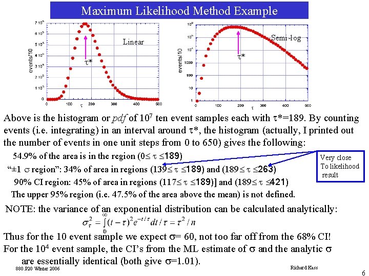
Maximum Likelihood Method Example Semi-log Linear t* t* Above is the histogram or pdf of 107 ten event samples each with t*=189. By counting events (i. e. integrating) in an interval around t*, the histogram (actually, I printed out the number of events in one unit steps from 0 to 650) gives the following: 54. 9% of the area is in the region (0£ t £ 189) “± 1 s region”: 34% of area in regions (139£ t £ 189) and (189£ t £ 263) 90% CI region: 45% of area in regions (117£ t £ 189)] and (189£ t £ 421) The upper 95% region (i. e. 47. 5% of the area above the mean) is not defined. Very close To likelihood result NOTE: the variance of an exponential distribution can be calculated analytically: Thus for the 10 event sample we expect s= 60, not too far off from the 68% CI! For the 104 event sample, the CI’s from the ML estimate of s and the analytic s are essentially identical (both give s=1. 01). 880. P 20 Winter 2006 Richard Kass 6

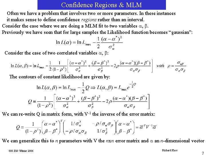
Confidence Regions & MLM Often we have a problem that involves two or more parameters. In these instances it makes sense to define confidence regions rather than an interval. Consider the case where we are doing a MLM fit to two variables a, b. Previously we have seen that for large samples the Likelihood function becomes “gaussian”: Consider the case of two correlated variables a, b: The contours of constant likelihood are given by: We can re-write Q in matrix form, with V-1 the inverse of the error matrix: We can generalize this to n parameters with V the nxn error matrix and a an n-dimensional vector 880. P 20 Winter 2006 Richard Kass 7

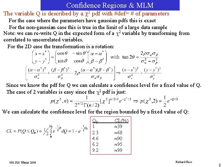
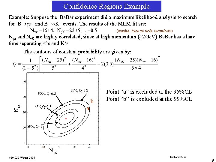
Confidence Regions & MLM The variable Q is described by a c 2 pdf with #dof= # of parameters For the case where the parameters have gaussian pdfs this is exact For the non-gaussian case this is true in the limit of a large data sample Note: we can re-write Q in the expected form of a c 2 variable by transforming from correlated to uncorrelated variables. For the 2 D case the transformation is a rotation: Since we know the pdf for Q we can calculate a confidence level for a fixed value of Q. The case of 2 variables is easy since the c 2 pdf is just: We can calculate the confidence level for the region bounded by a fixed value of Q: Q 0 1 2. 3 4. 6 6. 2 9. 2 880. P 20 Winter 2006 CL(%) » 39 » 68 » 90 » 95 » 99 Richard Kass 8

Confidence Regions Example: Suppose the Ba. Bar experiment did a maximum likelihood analysis to search for B®gp- and B®g. K- events. The results of the MLM fit are: Ngp =16± 4, Ng. K =25± 5, r=0. 5 (warning: these are made up numbers!) Ngp and Ng. K are highly correlated, since at high momentum (>2 Ge. V) Ba. Bar has a hard time separating p’s and K’s. The contours of constant probability are given by: 99%, Q=9. 2 95%, Q=6. 2 Ngp b Point “a” is excluded at the 95%CL Point “b” is excluded at the 99%CL a 68%, Q=2. 3 · 39%, Q=1 Ng. K 880. P 20 Winter 2006 Richard Kass 9

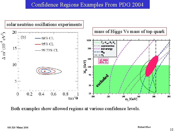
Confidence Regions Examples From PDG 2004 solar neutrino oscillations experiments mass of Higgs Vs mass of top quark Both examples show allowed regions at various confidence levels. 880. P 20 Winter 2006 Richard Kass 10