9 Confidence intervals Confidence intervals Point estimation The

9 Confidence intervals

Confidence intervals Point estimation The first method involves using the sample mean to estimate population mean Point estimation does not provide any information about the variability of the estimator, we do not know how close sample mean is to population mean Second method of estimation, known as interval estimation Range of values is called a confidence interval (CI) Chapter 9 p 218

9. 1 Two-sided confidence intervals Given a random variable X, the central limit theorem states that has a standard normal distribution (SND) if X is itself ND and an approximate SND if it is not but n is sufficiently large. 95% of the observations lie between -1. 96 and 1. 96, that is P(-1. 96≦Z ≦ 1. 96) = 0. 95 Substituting Z, rearranging the terms, We are 95% confident that the interval will cover m. Since the estimator is a random variable, therefore, the interval is random and has a 95% chance of covering m.

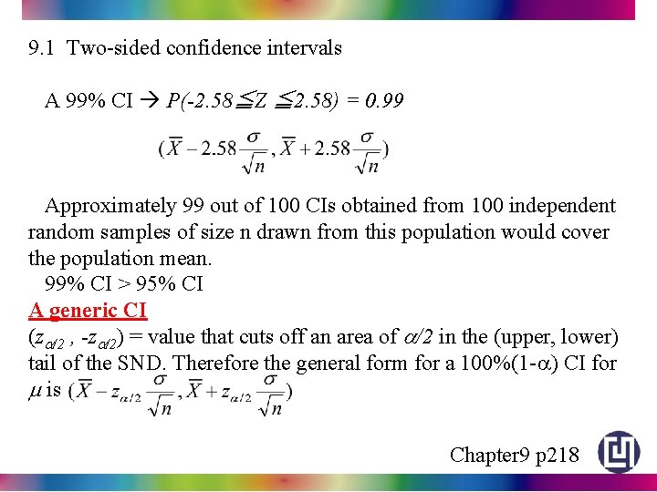
9. 1 Two-sided confidence intervals A 99% CI P(-2. 58≦Z ≦ 2. 58) = 0. 99 Approximately 99 out of 100 CIs obtained from 100 independent random samples of size n drawn from this population would cover the population mean. 99% CI > 95% CI A generic CI (za/2 , -za/2) = value that cuts off an area of a/2 in the (upper, lower) tail of the SND. Therefore the general form for a 100%(1 -a) CI for m is Chapter 9 p 218

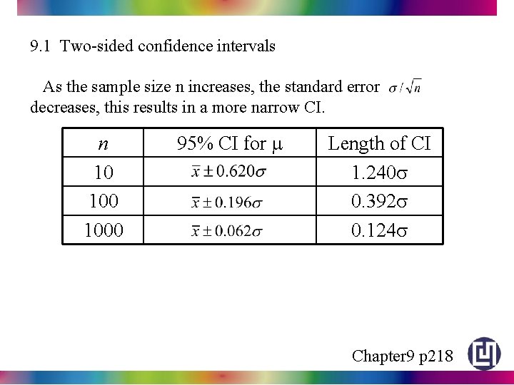
9. 1 Two-sided confidence intervals As the sample size n increases, the standard error decreases, this results in a more narrow CI. n 10 1000 95% CI for m Length of CI 1. 240 s 0. 392 s 0. 124 s Chapter 9 p 218

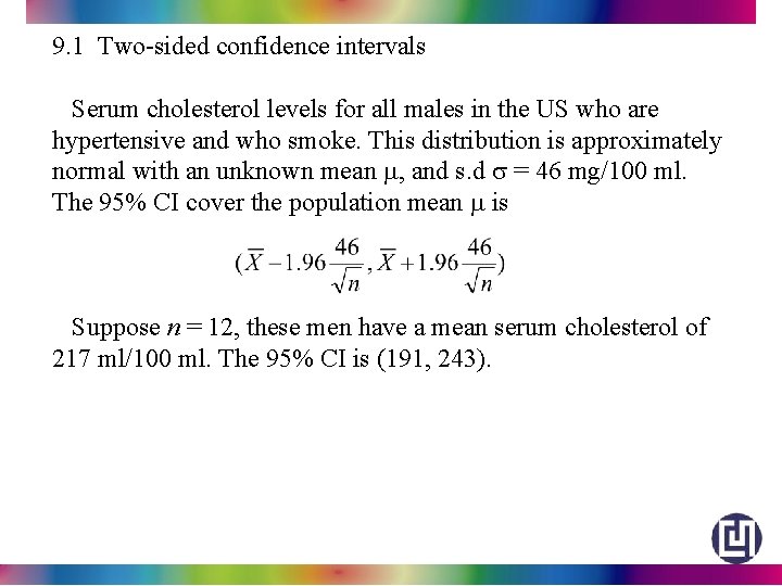
9. 1 Two-sided confidence intervals Serum cholesterol levels for all males in the US who are hypertensive and who smoke. This distribution is approximately normal with an unknown mean m, and s. d s = 46 mg/100 ml. The 95% CI cover the population mean m is Suppose n = 12, these men have a mean serum cholesterol of 217 ml/100 ml. The 95% CI is (191, 243).

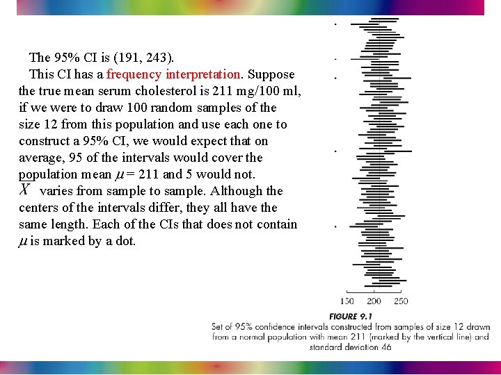
The 95% CI is (191, 243). This CI has a frequency interpretation. Suppose the true mean serum cholesterol is 211 mg/100 ml, if we were to draw 100 random samples of the size 12 from this population and use each one to construct a 95% CI, we would expect that on average, 95 of the intervals would cover the population mean m = 211 and 5 would not. varies from sample to sample. Although the centers of the intervals differ, they all have the same length. Each of the CIs that does not contain m is marked by a dot.

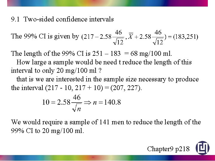
9. 1 Two-sided confidence intervals The 99% CI is given by The length of the 99% CI is 251 – 183 = 68 mg/100 ml. How large a sample would be need t reduce the length of this interval to only 20 mg/100 ml ? that is we are interested in the sample size necessary to produce the interval (217 - 10, 217 + 10) = (207, 227). We would require a sample of 141 men to reduce the length of the 99% CI to 20 mg/100 ml. Chapter 9 p 218

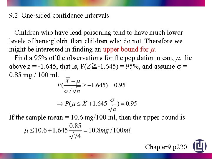
9. 2 One-sided confidence intervals Children who have lead poisoning tend to have much lower levels of hemoglobin than children who do not. Therefore we might be interested in finding an upper bound for m. Find a 95% of the observations for the population mean, m, lie above z = -1. 645, that is, P(Z≧-1. 645) = 95%, and assume s = 0. 85 mg / 100 ml. If the sample mean = 10. 6 mg/100 ml, then the upper bound is Chapter 9 p 220

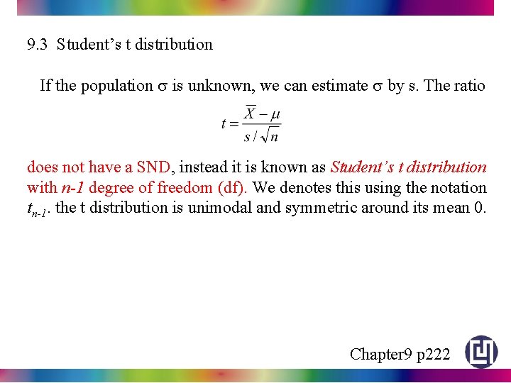
9. 3 Student’s t distribution If the population s is unknown, we can estimate s by s. The ratio does not have a SND, instead it is known as Student’s t distribution with n-1 degree of freedom (df). We denotes this using the notation tn-1. the t distribution is unimodal and symmetric around its mean 0. Chapter 9 p 222

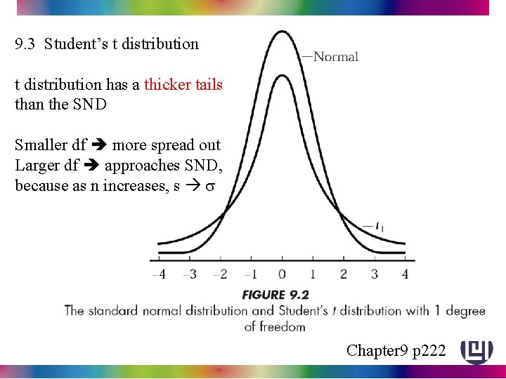
9. 3 Student’s t distribution has a thicker tails than the SND Smaller df more spread out Larger df approaches SND, because as n increases, s s Chapter 9 p 222

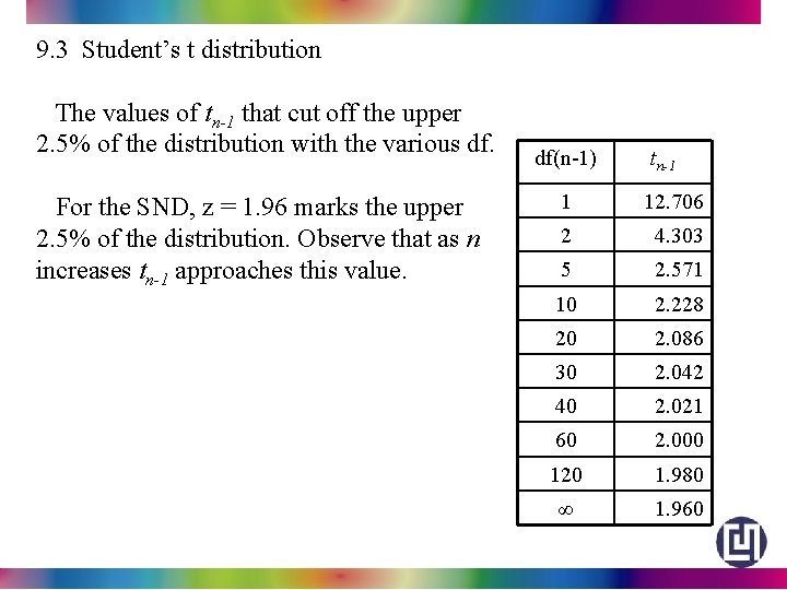
9. 3 Student’s t distribution The values of tn-1 that cut off the upper 2. 5% of the distribution with the various df. For the SND, z = 1. 96 marks the upper 2. 5% of the distribution. Observe that as n increases tn-1 approaches this value. df(n-1) tn-1 1 12. 706 2 4. 303 5 2. 571 10 2. 228 20 2. 086 30 2. 042 40 2. 021 60 2. 000 120 1. 980 ∞ 1. 960

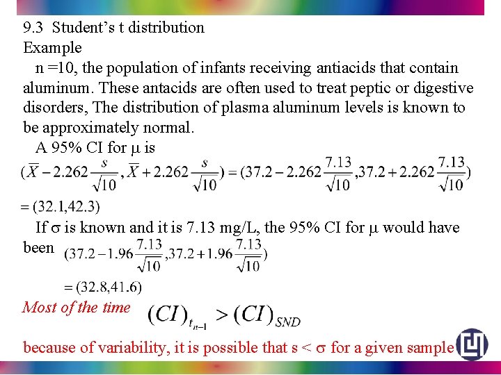
9. 3 Student’s t distribution Example n =10, the population of infants receiving antiacids that contain aluminum. These antacids are often used to treat peptic or digestive disorders, The distribution of plasma aluminum levels is known to be approximately normal. A 95% CI for m is If s is known and it is 7. 13 mg/L, the 95% CI for m would have been Most of the time because of variability, it is possible that s < s for a given sample

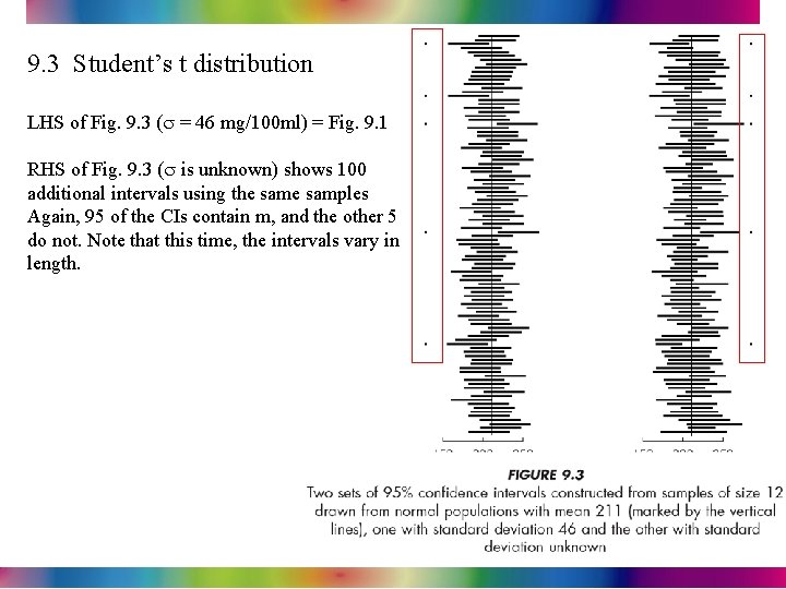
9. 3 Student’s t distribution LHS of Fig. 9. 3 (s = 46 mg/100 ml) = Fig. 9. 1 RHS of Fig. 9. 3 (s is unknown) shows 100 additional intervals using the samples Again, 95 of the CIs contain m, and the other 5 do not. Note that this time, the intervals vary in length. Chapter 9 p 224

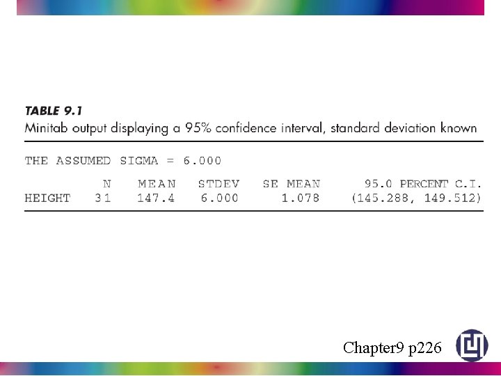
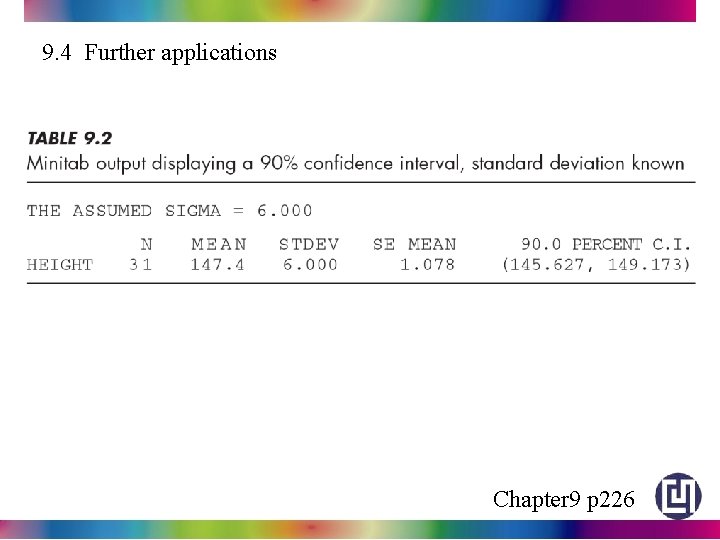
Chapter 9 p 226

9. 4 Further applications Chapter 9 p 226

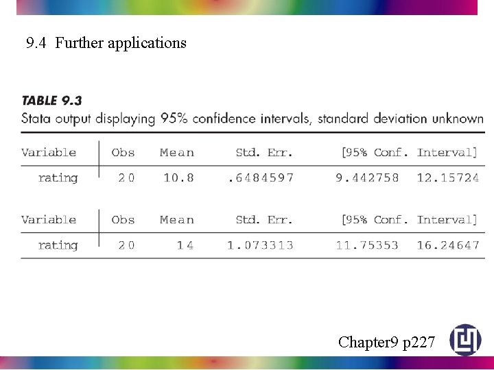
9. 4 Further applications Chapter 9 p 227