Confidence Intervals 1 a100 Confidence Intervals 1 Mean

Confidence Intervals

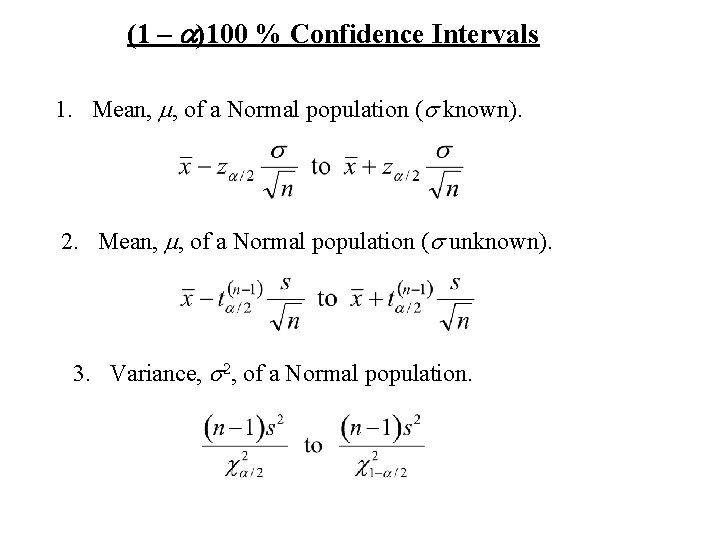
(1 – a)100 % Confidence Intervals 1. Mean, m, of a Normal population (s known). 2. Mean, m, of a Normal population (s unknown). 3. Variance, s 2, of a Normal population.

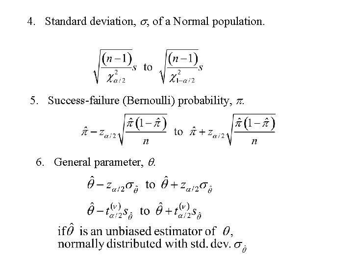
4. Standard deviation, s, of a Normal population. 5. Success-failure (Bernoulli) probability, p. 6. General parameter, q.

Hypothesis Testing An important area of statistical inference

Definition Hypothesis (H) – Statement about the parameters of the population • In hypothesis testing there are two hypotheses of interest. – The null hypothesis (H 0) – The alternative hypothesis (HA)

Either – null hypothesis (H 0) is true or – the alternative hypothesis (HA) is true. But not both We say that are mutually exclusive and exhaustive.

One has to make a decision – to either to accept null hypothesis (equivalent to rejecting HA) or – to reject null hypothesis (equivalent to accepting HA)

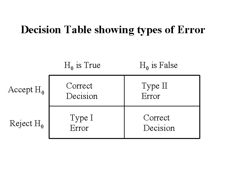
There are two possible errors that can be made. 1. Rejecting the null hypothesis when it is true. (type I error) 2. accepting the null hypothesis when it is false (type II error)

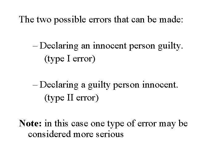
An analogy – a jury trial The two possible decisions are – Declare the accused innocent. – Declare the accused guilty.

The null hypothesis (H 0) – the accused is innocent The alternative hypothesis (HA) – the accused is guilty

The two possible errors that can be made: – Declaring an innocent person guilty. (type I error) – Declaring a guilty person innocent. (type II error) Note: in this case one type of error may be considered more serious

Decision Table showing types of Error H 0 is True H 0 is False Accept H 0 Correct Decision Type II Error Reject H 0 Type I Error Correct Decision

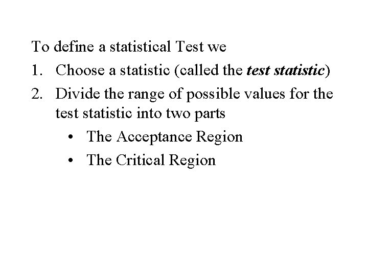
To define a statistical Test we 1. Choose a statistic (called the test statistic) 2. Divide the range of possible values for the test statistic into two parts • The Acceptance Region • The Critical Region

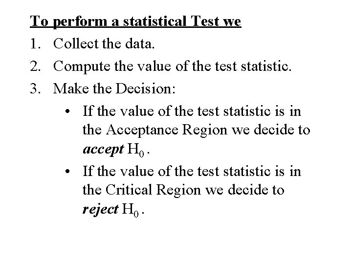
To perform a statistical Test we 1. Collect the data. 2. Compute the value of the test statistic. 3. Make the Decision: • If the value of the test statistic is in the Acceptance Region we decide to accept H 0. • If the value of the test statistic is in the Critical Region we decide to reject H 0.

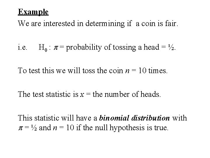
Example We are interested in determining if a coin is fair. i. e. H 0 : p = probability of tossing a head = ½. To test this we will toss the coin n = 10 times. The test statistic is x = the number of heads. This statistic will have a binomial distribution with p = ½ and n = 10 if the null hypothesis is true.

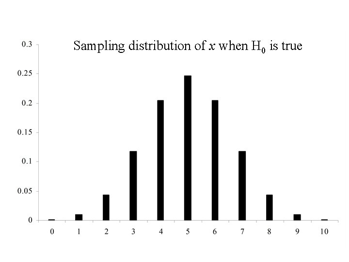
Sampling distribution of x when H 0 is true

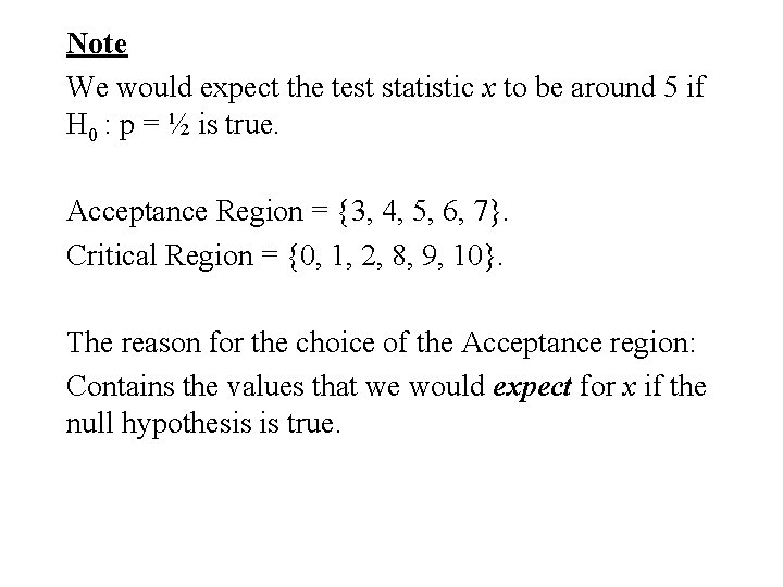
Note We would expect the test statistic x to be around 5 if H 0 : p = ½ is true. Acceptance Region = {3, 4, 5, 6, 7}. Critical Region = {0, 1, 2, 8, 9, 10}. The reason for the choice of the Acceptance region: Contains the values that we would expect for x if the null hypothesis is true.

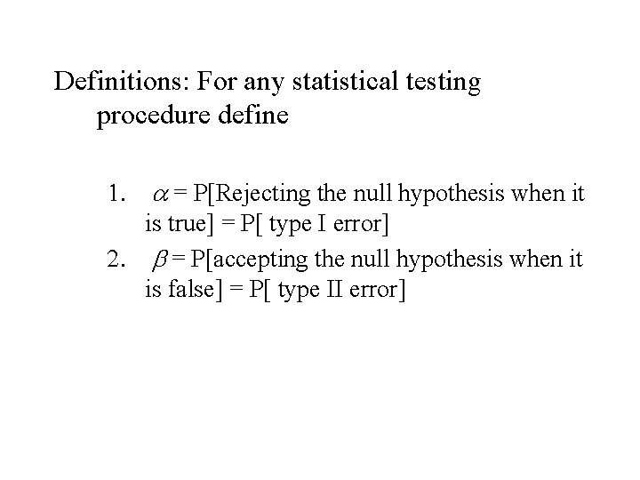
Definitions: For any statistical testing procedure define 1. a = P[Rejecting the null hypothesis when it is true] = P[ type I error] 2. b = P[accepting the null hypothesis when it is false] = P[ type II error]

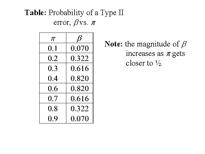
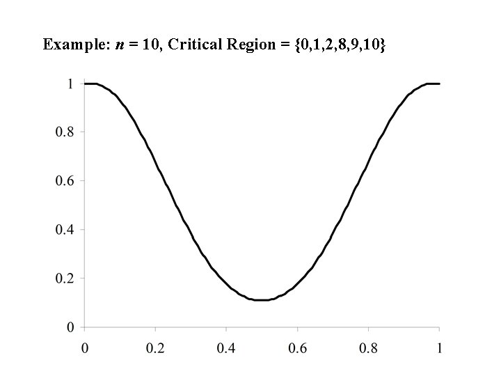
In the last example 1. a = P[ type I error] = p(0) + p(1) + p(2) + p(8) + p(9) + p(10) = 0. 109, where p(x) are binomial probabilities with p = ½ and n = 10. 2. b = P[ type II error] = p(3) + p(4) + p(5) + p(6) + p(7), where p(x) are binomial probabilities with p (not equal to ½) and n = 10. Note: these will depend on the value of p.

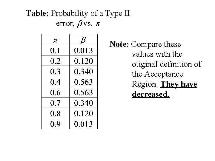
Table: Probability of a Type II error, b vs. p Note: the magnitude of b increases as p gets closer to ½.

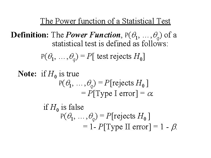
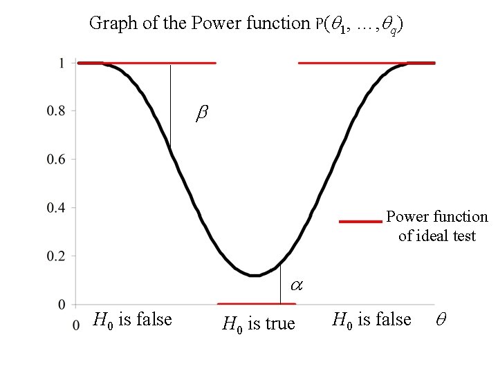
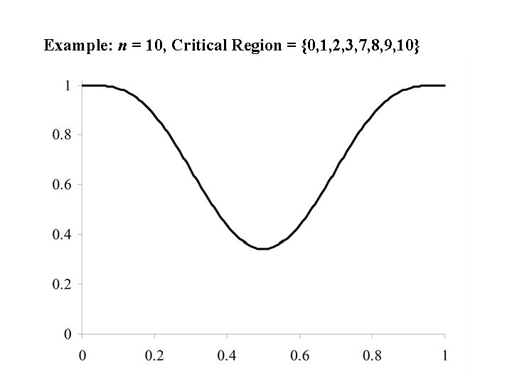
The Power function of a Statistical Test Definition: The Power Function, P(q 1, …, qq) of a statistical test is defined as follows: P(q 1, …, qq) = P[ test rejects H 0] Note: if H 0 is true P(q 1, …, qq) = P[rejects H 0 ] = P[Type I error] = a. if H 0 is false P(q 1, …, qq) = P[rejects H 0 ] = 1 - P[Type II error] = 1 - b.

Graph of the Power function P(q 1, …, qq) b Power function of ideal test a H 0 is false H 0 is true H 0 is false q

Example: n = 10, Critical Region = {0, 1, 2, 8, 9, 10}

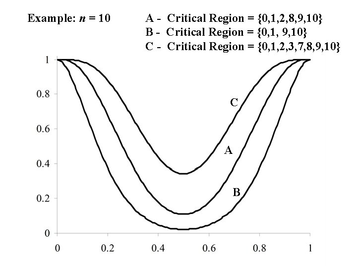
Comments: 1. You can control a = P[ type I error] and b = P[ type II error] by widening or narrowing the acceptance region. . 2. Widening the acceptance region decreases a = P[ type I error] but increases b = P[ type II error]. 3. Narrowing the acceptance region increases a = P[ type I error] but decreases b = P[ type II error].

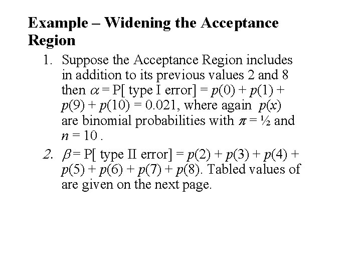
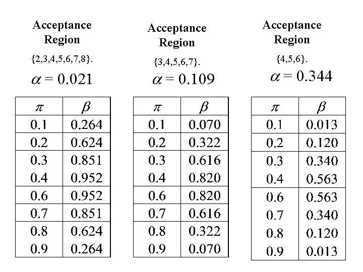
Example – Widening the Acceptance Region 1. Suppose the Acceptance Region includes in addition to its previous values 2 and 8 then a = P[ type I error] = p(0) + p(1) + p(9) + p(10) = 0. 021, where again p(x) are binomial probabilities with p = ½ and n = 10. 2. b = P[ type II error] = p(2) + p(3) + p(4) + p(5) + p(6) + p(7) + p(8). Tabled values of are given on the next page.

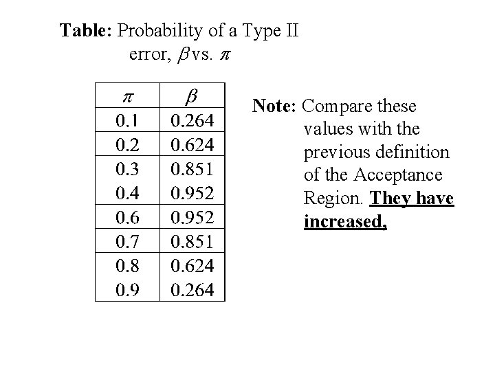
Table: Probability of a Type II error, b vs. p Note: Compare these values with the previous definition of the Acceptance Region. They have increased,

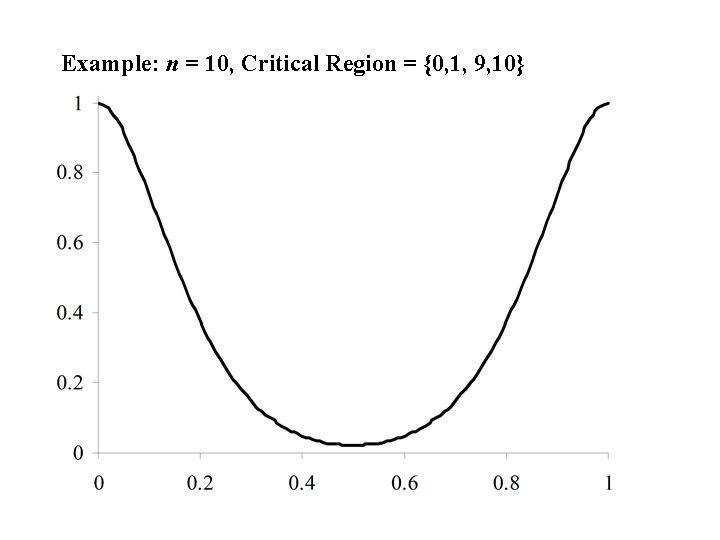
Example: n = 10, Critical Region = {0, 1, 9, 10}

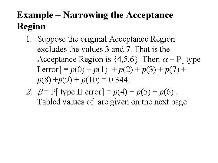
Example – Narrowing the Acceptance Region 1. Suppose the original Acceptance Region excludes the values 3 and 7. That is the Acceptance Region is {4, 5, 6}. Then a = P[ type I error] = p(0) + p(1) + p(2) + p(3) + p(7) + p(8) +p(9) + p(10) = 0. 344. 2. b = P[ type II error] = p(4) + p(5) + p(6). Tabled values of are given on the next page.

Table: Probability of a Type II error, b vs. p Note: Compare these values with the otiginal definition of the Acceptance Region. They have decreased,

Example: n = 10, Critical Region = {0, 1, 2, 3, 7, 8, 9, 10}

Acceptance Region {2, 3, 4, 5, 6, 7, 8}. {3, 4, 5, 6, 7}. {4, 5, 6}. a = 0. 021 a = 0. 109 a = 0. 344

Example: n = 10 A - Critical Region = {0, 1, 2, 8, 9, 10} B - Critical Region = {0, 1, 9, 10} C - Critical Region = {0, 1, 2, 3, 7, 8, 9, 10} C A B

The Approach in Statistical Testing is: • Set up the Acceptance Region so that a is close to some predetermine value (the usual values are 0. 05 or 0. 01) • The predetermine value of a (0. 05 or 0. 01) is called the significance level of the test. • The significance level (size) of the test is a = P[test makes a type I error]

The z-test for the Mean of a Normal Population We want to test, m, denote the mean of a normal population

The t distribution Estimating m, the mean of a Normal population (s 2 unknown) Let x 1, … , xn denote a sample from the normal distribution with mean m and variance s 2. Both m and s 2 are unknown Recall Also

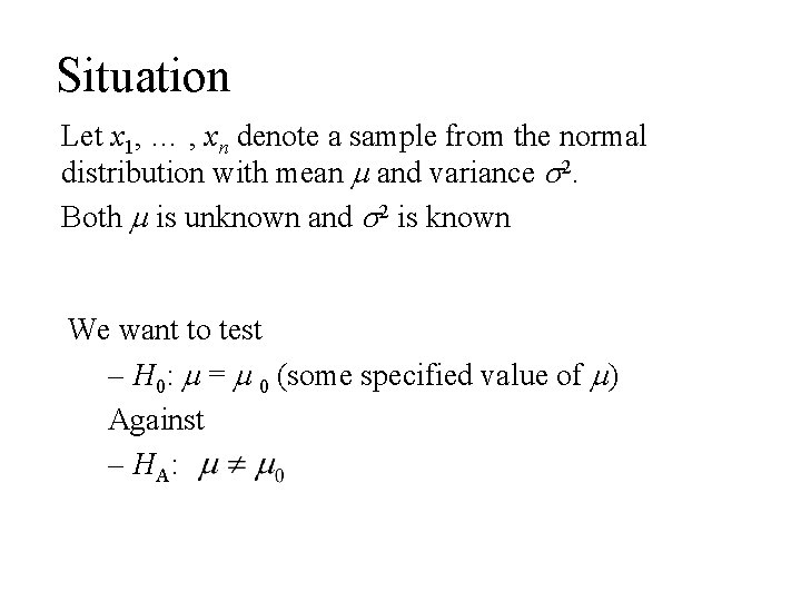
Situation Let x 1, … , xn denote a sample from the normal distribution with mean m and variance s 2. Both m is unknown and s 2 is known We want to test – H 0: m = m 0 (some specified value of m) Against – H A:

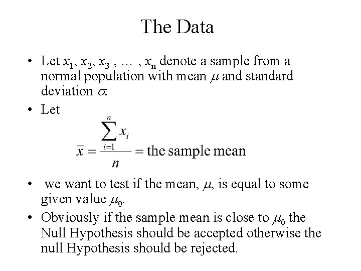
The Data • Let x 1, x 2, x 3 , … , xn denote a sample from a normal population with mean m and standard deviation s. • Let • we want to test if the mean, m, is equal to some given value m 0. • Obviously if the sample mean is close to m 0 the Null Hypothesis should be accepted otherwise the null Hypothesis should be rejected.

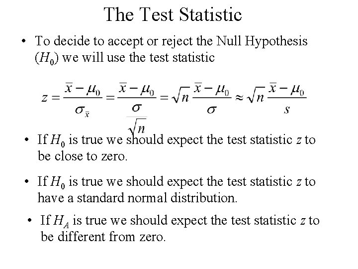
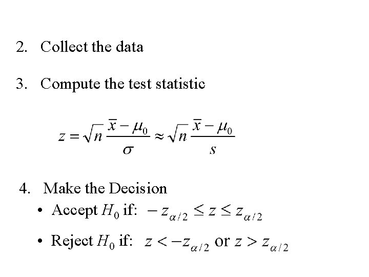
The Test Statistic • To decide to accept or reject the Null Hypothesis (H 0) we will use the test statistic • If H 0 is true we should expect the test statistic z to be close to zero. • If H 0 is true we should expect the test statistic z to have a standard normal distribution. • If HA is true we should expect the test statistic z to be different from zero.

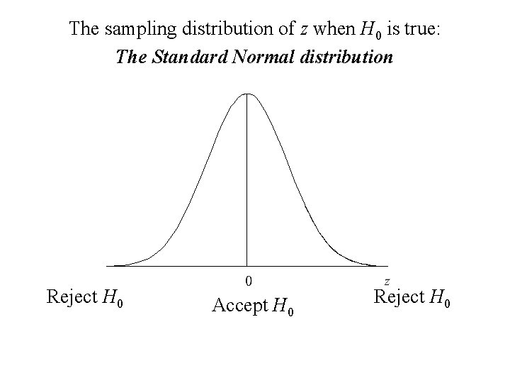
The sampling distribution of z when H 0 is true: The Standard Normal distribution Reject H 0 Accept H 0 Reject H 0

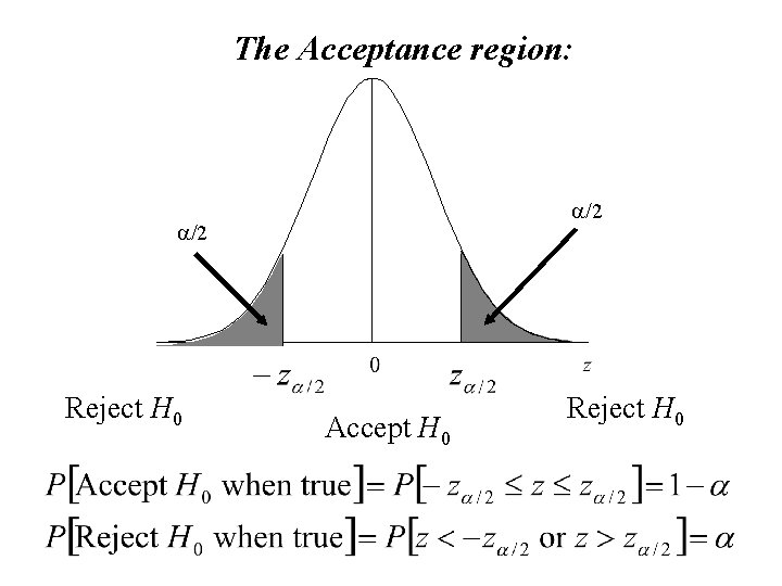
The Acceptance region: a/2 Reject H 0 Accept H 0 Reject H 0

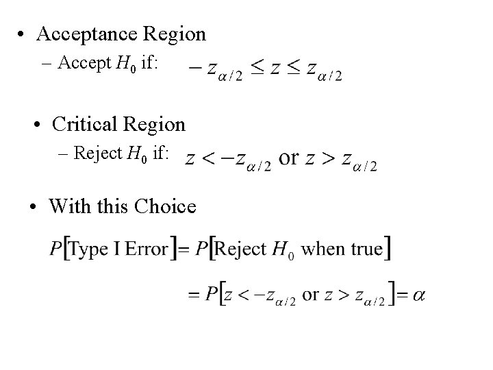
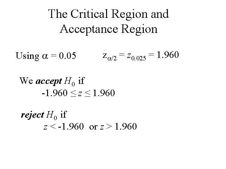
• Acceptance Region – Accept H 0 if: • Critical Region – Reject H 0 if: • With this Choice

Summary To Test for a binomial probability m H 0: m = m 0 (some specified value of m) Against H A: 1. Decide on a = P[Type I Error] = the significance level of the test (usual choices 0. 05 or 0. 01)

2. Collect the data 3. Compute the test statistic 4. Make the Decision • Accept H 0 if: • Reject H 0 if:

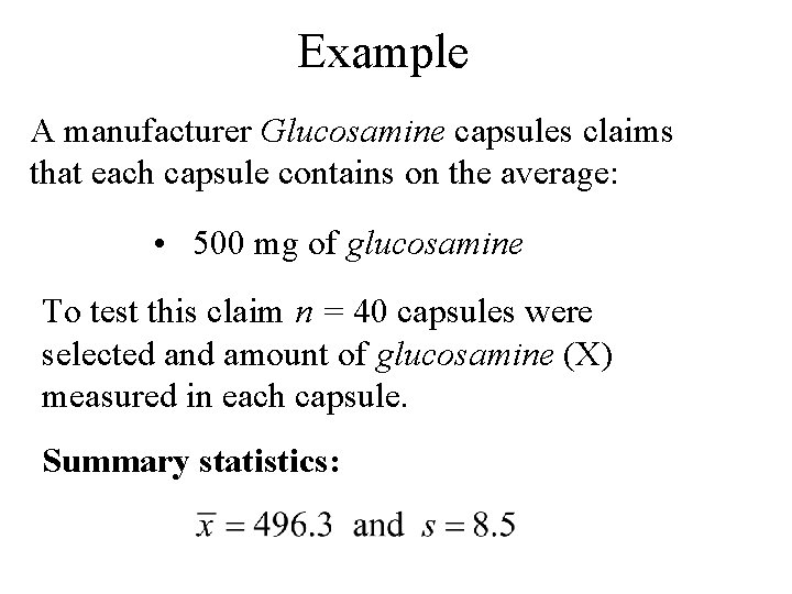
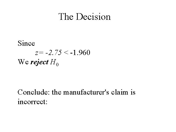
Example A manufacturer Glucosamine capsules claims that each capsule contains on the average: • 500 mg of glucosamine To test this claim n = 40 capsules were selected and amount of glucosamine (X) measured in each capsule. Summary statistics:

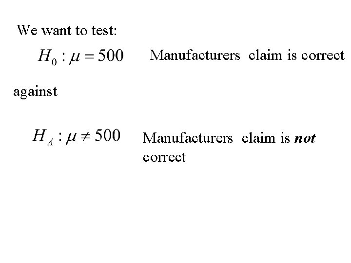
We want to test: Manufacturers claim is correct against Manufacturers claim is not correct

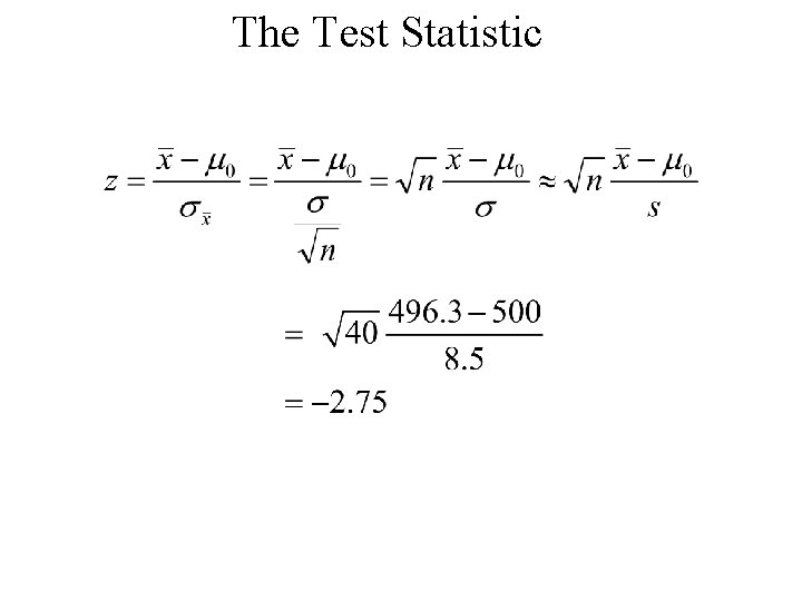
The Test Statistic

The Critical Region and Acceptance Region Using a = 0. 05 za/2 = z 0. 025 = 1. 960 We accept H 0 if -1. 960 ≤ z ≤ 1. 960 reject H 0 if z < -1. 960 or z > 1. 960

The Decision Since z= -2. 75 < -1. 960 We reject H 0 Conclude: the manufacturer's claim is incorrect: