Computer Graphics Modeling 1 Modeling Modeling is simply

Computer Graphics Modeling 1

Modeling • Modeling is simply the process of creating 3 D objects – Many different processes to create models – Many different representations of model data • Once the models are obtained, one can transform them to the correct locations in space, place a virtual camera in space, and render a 2 D image of the scene 2

Model Representations • • • Polygonal CSG (constructive solid geometry) Spatial subdivision techniques Implicit representation Parametric patches 3

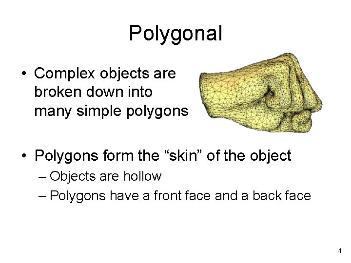
Polygonal • Complex objects are broken down into many simple polygons • Polygons form the “skin” of the object – Objects are hollow – Polygons have a front face and a back face 4

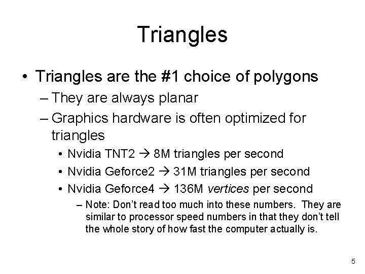
Triangles • Triangles are the #1 choice of polygons – They are always planar – Graphics hardware is often optimized for triangles • Nvidia TNT 2 8 M triangles per second • Nvidia Geforce 2 31 M triangles per second • Nvidia Geforce 4 136 M vertices per second – Note: Don’t read too much into these numbers. They are similar to processor speed numbers in that they don’t tell the whole story of how fast the computer actually is. 5

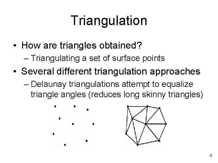
Triangulation • How are triangles obtained? – Triangulating a set of surface points • Several different triangulation approaches – Delaunay triangulations attempt to equalize triangles (reduces long skinny triangles) 6

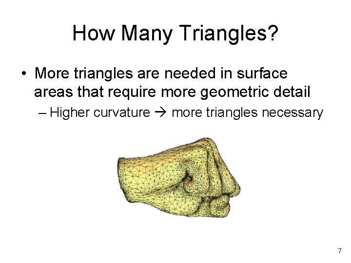
How Many Triangles? • More triangles are needed in surface areas that require more geometric detail – Higher curvature more triangles necessary 7

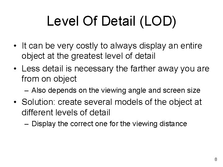
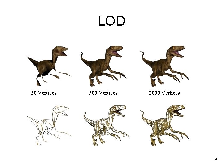
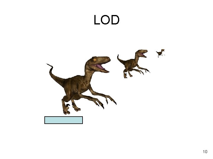
Level Of Detail (LOD) • It can be very costly to always display an entire object at the greatest level of detail • Less detail is necessary the farther away you are from on object – Also depends on the viewing angle and screen size • Solution: create several models of the object at different levels of detail – Display the correct one for the viewing distance 8

LOD 50 Vertices 500 Vertices 2000 Vertices 9

LOD 10

LOD • How to create the same model in multiple levels of detail? – Ex: start with most detailed, resample with less vertices, and then re-triangulate • When to switch models when rendering? – Based on distance and screen size – Ex: 640 x 480 screen 307, 200 pixels Object takes up half of screen 150 K pixels Any more than 300 K triangles (half are facing away from the camera) is overkill at this distance and screen size – Visual artifacts can occur at switching point 11

Creating the Surface Points • Triangulation works on a set of points – One needs to create this surface point set • Many different approaches: – Manual placement – Mathematical (geometrical) generation – Scanning real objects 12

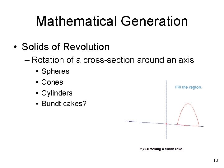
Mathematical Generation • Solids of Revolution – Rotation of a cross-section around an axis • • Spheres Cones Cylinders Bundt cakes? 13

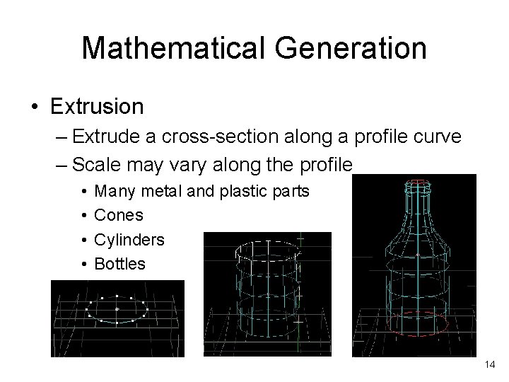
Mathematical Generation • Extrusion – Extrude a cross-section along a profile curve – Scale may vary along the profile • • Many metal and plastic parts Cones Cylinders Bottles 14

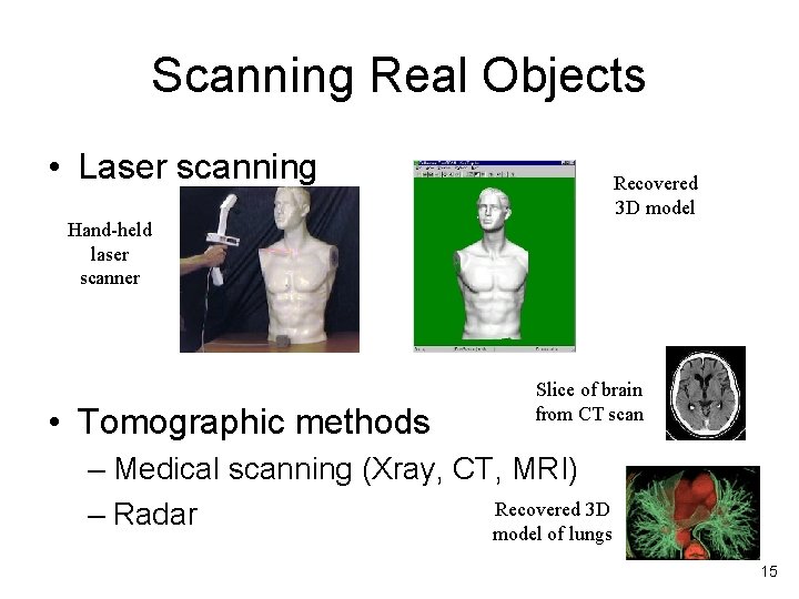
Scanning Real Objects • Laser scanning Recovered 3 D model Hand-held laser scanner • Tomographic methods Slice of brain from CT scan – Medical scanning (Xray, CT, MRI) Recovered 3 D – Radar model of lungs 15

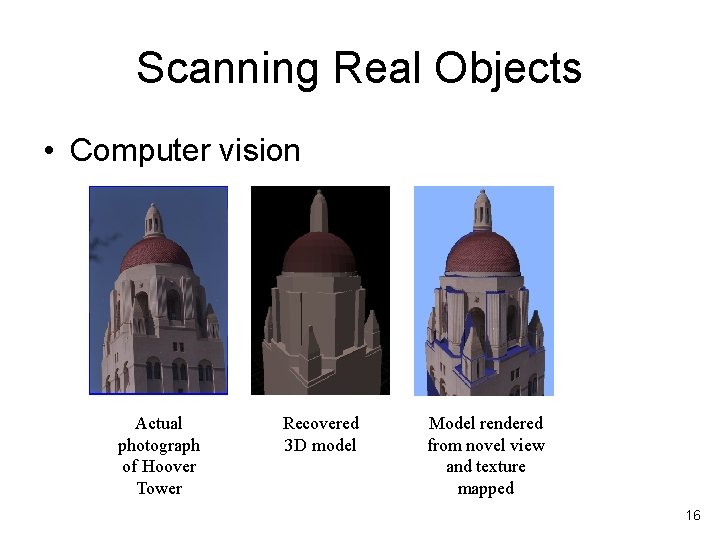
Scanning Real Objects • Computer vision Actual photograph of Hoover Tower Recovered 3 D model Model rendered from novel view and texture mapped 16

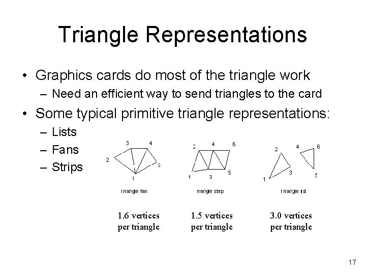
Triangle Representations • Graphics cards do most of the triangle work – Need an efficient way to send triangles to the card • Some typical primitive triangle representations: – Lists – Fans – Strips 1. 6 vertices per triangle 1. 5 vertices per triangle 3. 0 vertices per triangle 17

Triangle Representations • Adding a level of indirection with indexed triangle representations – Store the vertices (in a vertex buffer) independently of the rendering order (which is stored in a index buffer) – Enables one to reuse a vertex multiple times without sending 3 coordinates each time • Conventional wisdom is that indexed triangle strips are the most efficient triangle representation 18

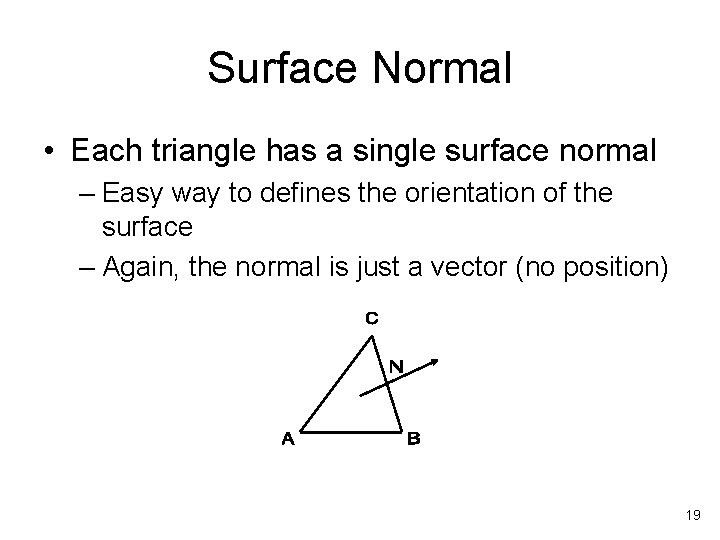
Surface Normal • Each triangle has a single surface normal – Easy way to defines the orientation of the surface – Again, the normal is just a vector (no position) 19

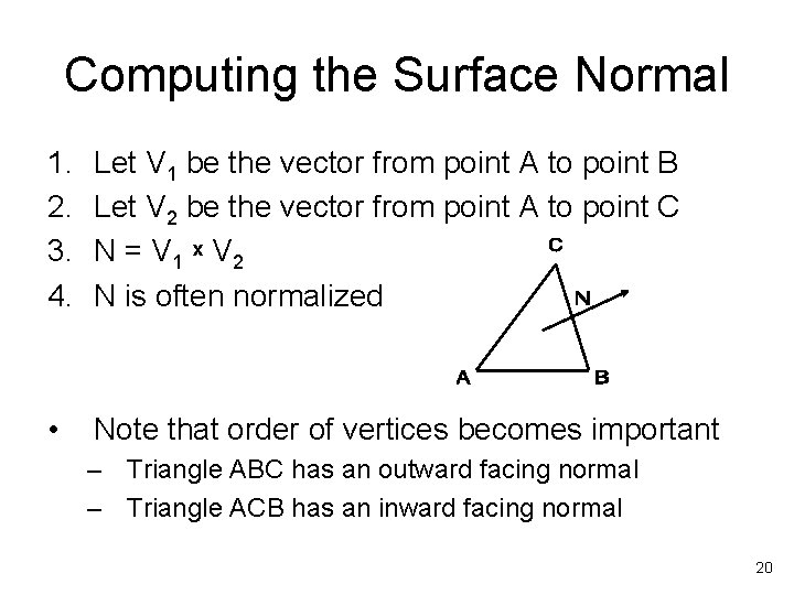
Computing the Surface Normal 1. 2. 3. 4. Let V 1 be the vector from point A to point B Let V 2 be the vector from point A to point C N = V 1 x V 2 N is often normalized • Note that order of vertices becomes important – Triangle ABC has an outward facing normal – Triangle ACB has an inward facing normal 20

Modeling Approaches • • • Polygonal CSG (constructive solid geometry) Spatial subdivision techniques Implicit representation Parametric patches 21

Constructive Solid Geometry • Unlike polygonal approaches, CSG models are “solids” – Polygonal models are “skins” • Solid approaches are often better suited for medical applications because – Cutting slices through objects – Representing internal functional data • Temperature • Blood flow 22

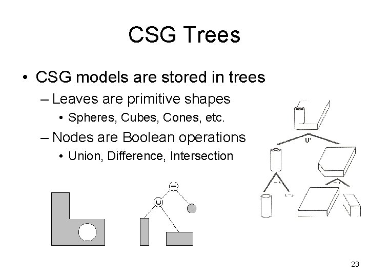
CSG Trees • CSG models are stored in trees – Leaves are primitive shapes • Spheres, Cubes, Cones, etc. – Nodes are Boolean operations • Union, Difference, Intersection 23

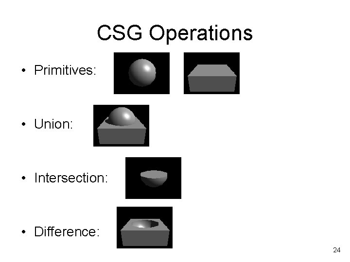
CSG Operations • Primitives: • Union: • Intersection: • Difference: 24

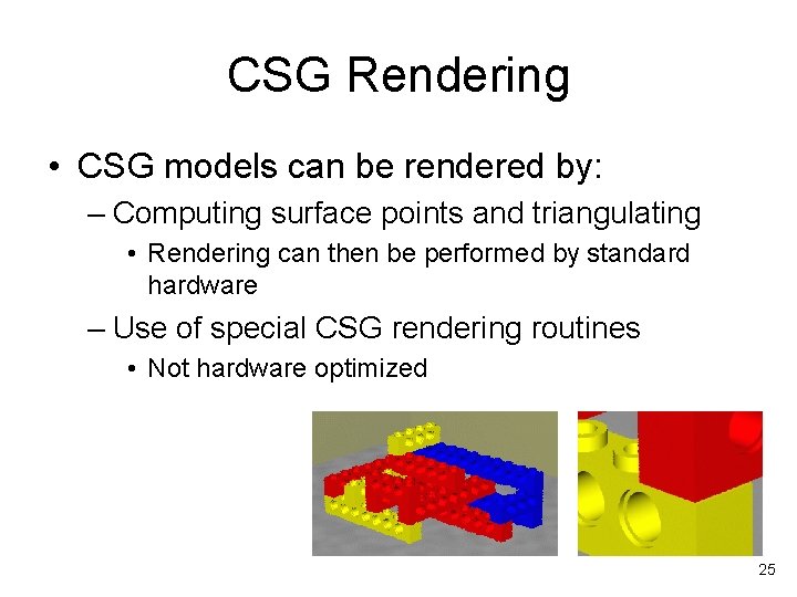
CSG Rendering • CSG models can be rendered by: – Computing surface points and triangulating • Rendering can then be performed by standard hardware – Use of special CSG rendering routines • Not hardware optimized 25

Modeling Approaches • • • Polygonal CSG (constructive solid geometry) Spatial subdivision techniques Implicit representation Parametric patches 26

Spatial subdivision techniques • The idea is to divide up space into pieces that are the object are pieces that are not the object – A “solid” approach to modeling • Usually pieces are cubes • Amount of detail that can be represented is controlled by how small the cubes are 27

2 D Images • B/W images – Image is evenly divided up into pixels – Pixels size controls the level of detail – Pixels are on/off to represent presence/absence of object – Representation designed for ease of blitting onto screen, not for efficient data representation 28

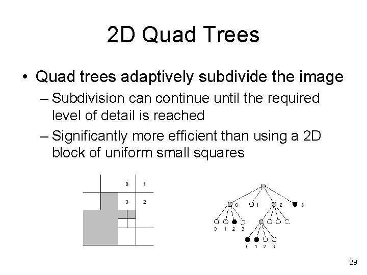
2 D Quad Trees • Quad trees adaptively subdivide the image – Subdivision can continue until the required level of detail is reached – Significantly more efficient than using a 2 D block of uniform small squares 29

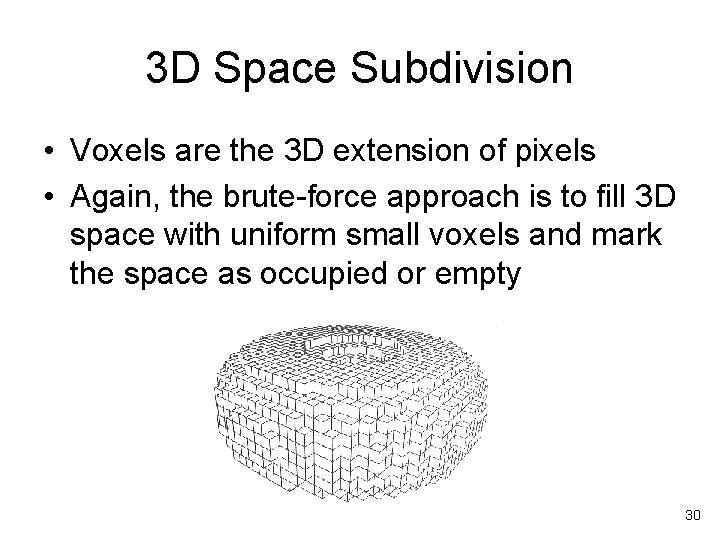
3 D Space Subdivision • Voxels are the 3 D extension of pixels • Again, the brute-force approach is to fill 3 D space with uniform small voxels and mark the space as occupied or empty 30

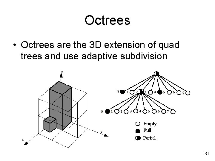
Octrees • Octrees are the 3 D extension of quad trees and use adaptive subdivision 31

Modeling Approaches • • • Polygonal CSG (constructive solid geometry) Spatial subdivision techniques Implicit representation Parametric patches 32

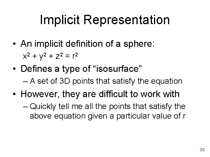
Implicit Representation • An implicit definition of a sphere: x 2 + y 2 + z 2 = r 2 • Defines a type of “isosurface” – A set of 3 D points that satisfy the equation • However, they are difficult to work with – Quickly tell me all the points that satisfy the above equation given a particular value of r 33

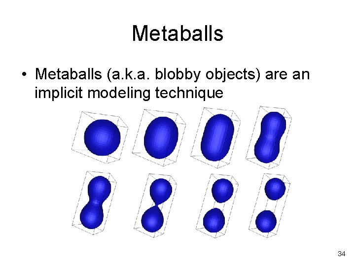
Metaballs • Metaballs (a. k. a. blobby objects) are an implicit modeling technique 34

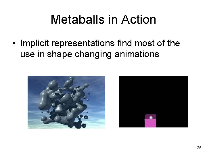
Metaballs in Action • Implicit representations find most of the use in shape changing animations 35

Modeling Approaches • • • Polygonal CSG (constructive solid geometry) Spatial subdivision techniques Implicit representation Parametric patches 36

Parametric Patches • Parametric patches are used to model smooth curved surfaces and to allow dynamic control over the shape of the surface • Parametric patches are uses heavily in CAD application and animation • Currently real-time applications are dominated by triangle meshes – Patches hold many advantages over triangle meshes and if hardware support for them becomes widespread there could be a major shift to them 37

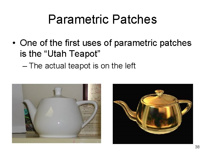
Parametric Patches • One of the first uses of parametric patches is the “Utah Teapot” – The actual teapot is on the left 38

Parametric Patches • We will start be examining curves – Bézier curves – B-Spline curves • Then we will expand to surface patches – Bézier patches – B-Spline patches 39

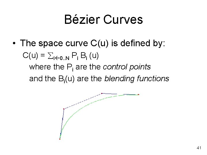
Bézier Curves • Pierre Bézier, a French designer, first used them in the 1970’s in the design of Renault car bodies • Since, they have been heavily used by Adobe in their fonts as well as in graphic applications • A Bézier curve is a parametric curve – The function C(u) defines the curve points (x, y, z) as the parameter u varies through [0. . 1] 40

Bézier Curves • The space curve C(u) is defined by: C(u) = i 0. . N Pi Bi (u) where the Pi are the control points and the Bi(u) are the blending functions 41

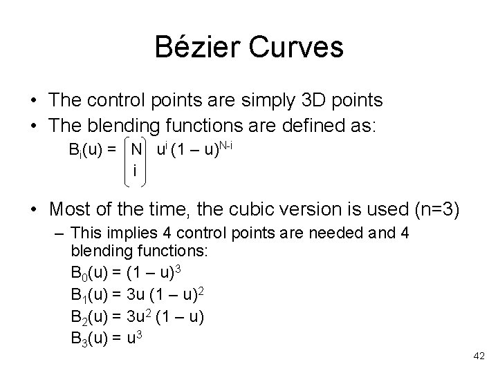
Bézier Curves • The control points are simply 3 D points • The blending functions are defined as: Bi(u) = N ui (1 – u)N-i i • Most of the time, the cubic version is used (n=3) – This implies 4 control points are needed and 4 blending functions: B 0(u) = (1 – u)3 B 1(u) = 3 u (1 – u)2 B 2(u) = 3 u 2 (1 – u) B 3(u) = u 3 42

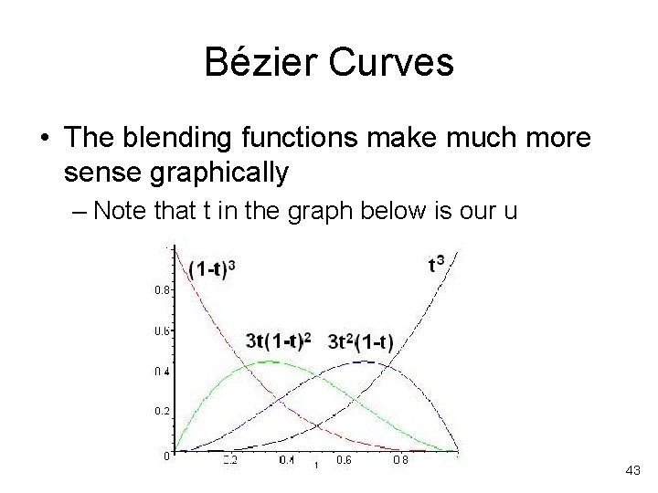
Bézier Curves • The blending functions make much more sense graphically – Note that t in the graph below is our u 43

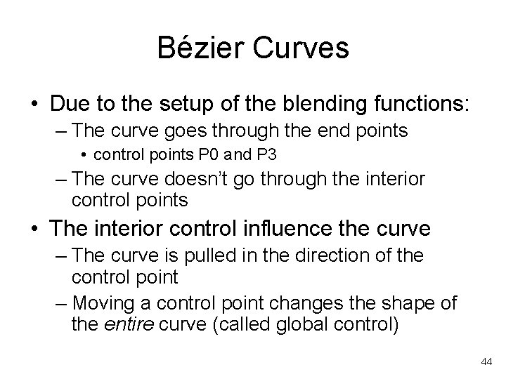
Bézier Curves • Due to the setup of the blending functions: – The curve goes through the end points • control points P 0 and P 3 – The curve doesn’t go through the interior control points • The interior control influence the curve – The curve is pulled in the direction of the control point – Moving a control point changes the shape of the entire curve (called global control) 44

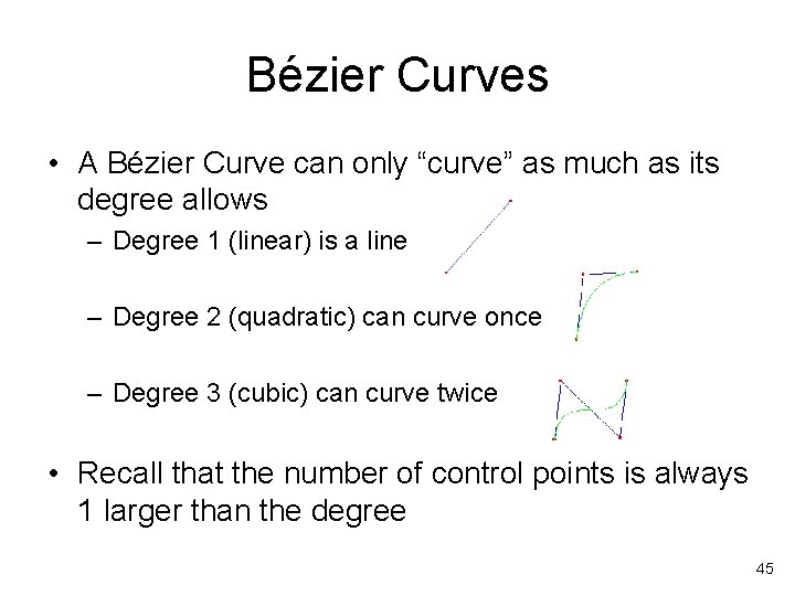
Bézier Curves • A Bézier Curve can only “curve” as much as its degree allows – Degree 1 (linear) is a line – Degree 2 (quadratic) can curve once – Degree 3 (cubic) can curve twice • Recall that the number of control points is always 1 larger than the degree 45

Bézier Curves • So what if you want a really “curvy” curve? – You could increase the degree of the curve • The downfall of this approach is that each control point has global control over the curve shape – That is, changing a single control point will modify the shape of the entire curve (not great for modeling) – High degree curves are “unstable” • It is computationally expensive – You could join multiple cubic curves together • Each control point only has influence over its piece of the curve (local control w. r. t. the entire joined curve) • Hardware can be optimized for cubic curves • But, we must maintain continuity across the joins! 46

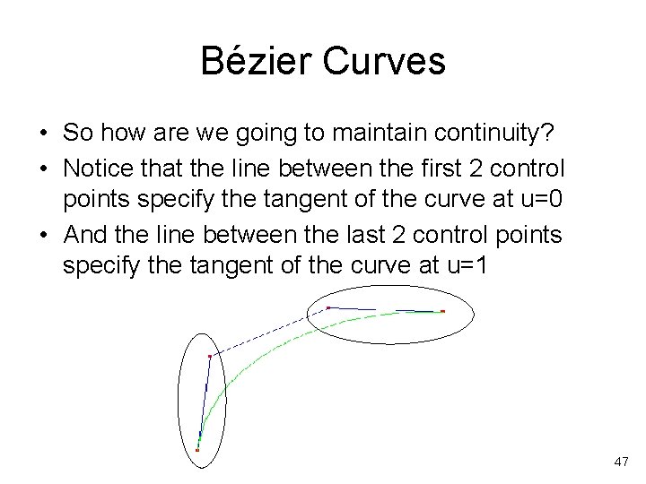
Bézier Curves • So how are we going to maintain continuity? • Notice that the line between the first 2 control points specify the tangent of the curve at u=0 • And the line between the last 2 control points specify the tangent of the curve at u=1 47

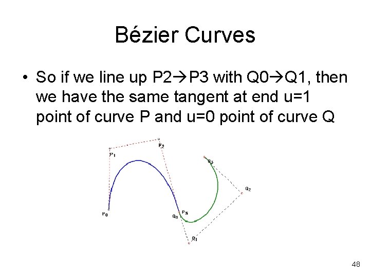
Bézier Curves • So if we line up P 2 P 3 with Q 0 Q 1, then we have the same tangent at end u=1 point of curve P and u=0 point of curve Q 48

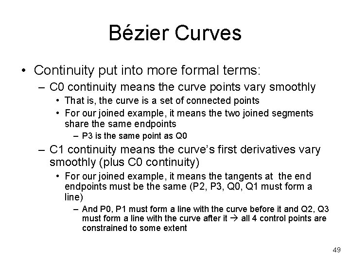
Bézier Curves • Continuity put into more formal terms: – C 0 continuity means the curve points vary smoothly • That is, the curve is a set of connected points • For our joined example, it means the two joined segments share the same endpoints – P 3 is the same point as Q 0 – C 1 continuity means the curve’s first derivatives vary smoothly (plus C 0 continuity) • For our joined example, it means the tangents at the endpoints must be the same (P 2, P 3, Q 0, Q 1 must form a line) – And P 0, P 1 must form a line with the curve before it and Q 2, Q 3 must form a line with the curve after it all 4 control points are constrained to some extent 49

Bézier Curves – C 2 continuity means the curve’s second derivatives vary smoothly (plus C 1 continuity) • Second derivative corresponds to curvature • For our joined example, it implies constrains on P 1, P 2, P 3, Q 0, Q 1, and Q 2 – Plus P 0, P 1, and P 2 are constrained from the curve before it and Q 1, Q 2, and Q 3 are constrained from the curve after it – Thus, although it can be achieved, there are so many constrains on the positions of the control points that joined cubic Bézier curves are almost never C 2 continuous 50

Bézier Curves • Do we care about C 2 continuity? – Probably not for simple modeling – But if the curve is being used to specify the path/orientation of a camera: • Not C 0 means the camera position jumps • Not C 1 means the camera’s orientation jumps • Not C 2 means the change in the camera’s orientation has sudden jumps – Think in terms of a car: position, velocity, acceleration 51

B-Spline Curves • B-Splines fix two major problems of Béziers: – Global control of control points – Relationship between degree of the curve and the number of control points • This is achieved by letting the user specify any number of control points and automatically constructing a set of cubic curves that are C 2 – This is similar to a set of joined cubic Bézier curves • Joined cubic Bézier curves can have any number of control points and are still cubic, and each control point only influences its local cubic curve – But B-Splines are C 2 and have no constraints on control point locations as joined cubic Bézier curves 52

B-Spline Curves • The definition of cubic B-Spline curve is: C(u) = i 0. . M Pi Bi (u) • So just like with Bézier curves, we have control points (Pi) and blending functions (Bi(u)) • However, a full B-Spline curve of M+1 control points is really made up of M-2 curve segments, each being controlled by 4 of the control points • Also, the blending functions are defined differently than with Bézier curves, with the two most popular variations being: – Uniform – Non-Uniform 53

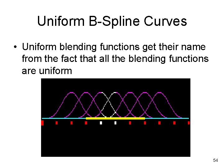
Uniform B-Spline Curves • Uniform blending functions get their name from the fact that all the blending functions are uniform 54

Uniform B-Spline Curves • Recall that each curve segment composing the full B-Spline needs 4 control points modified by 4 blending functions • This implies that only the section in yellow on the previous slide can be used to define the curve – At either end there are not enough blending functions • This also implies that the curve will not go through any of the control points, including the first and last (as was the case with Bézier) – There are multiple non-zero blending functions at u=0 and u=1 55

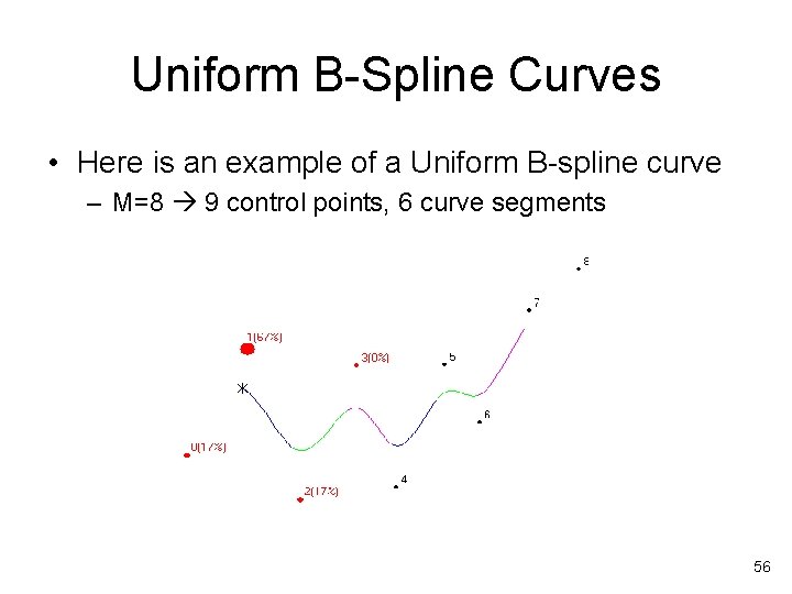
Uniform B-Spline Curves • Here is an example of a Uniform B-spline curve – M=8 9 control points, 6 curve segments 56

Non-Uniform B-Spline Curves • The main difference between Uniform and Non. Uniform B-Splines is that all the blending functions are not the same • There are several variations on the blending functions, all controlled by “knot values” – We won’t get into the details of knot values • In particular, the blending function can be specified in such a way as force the curve to go through the endpoints (like Bézier) – P. 97 from 3 D games book has a good example 57

Rational Curves • A rational curve is a curve defined in 4 D space that is then projected into 3 D space • The main point of using rational curves is that it allows you to define weights on the control points – Giving a control point a higher weight causes the curve to be pulled more towards that control point – P. 105 in 3 D games book for an example • One can have Rational Bézier curves or Rational B-Spline curves – Or other types of curves not covered (Hermite, etc. ) 58

NURBS • NURBS stands for Non-Uniform Rational BSplines • It is one of the most popular curve representations used in CAD and graphics work because it allows: – Local control of the curve when moving the control points (B-Spline) – Ability to adjust the blending functions by moving the “knot values” (Non-Uniform) – Ability to weight the control points (Rational) 59

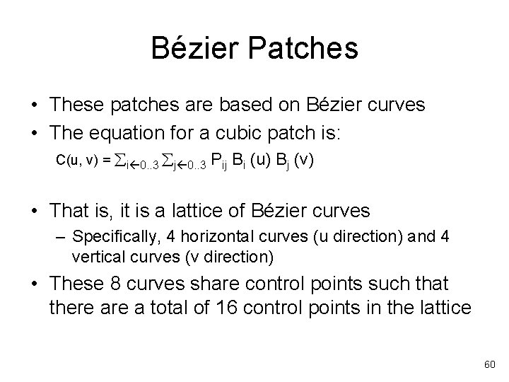
Bézier Patches • These patches are based on Bézier curves • The equation for a cubic patch is: C(u, v) = i 0. . 3 j 0. . 3 Pij Bi (u) Bj (v) • That is, it is a lattice of Bézier curves – Specifically, 4 horizontal curves (u direction) and 4 vertical curves (v direction) • These 8 curves share control points such that there a total of 16 control points in the lattice 60

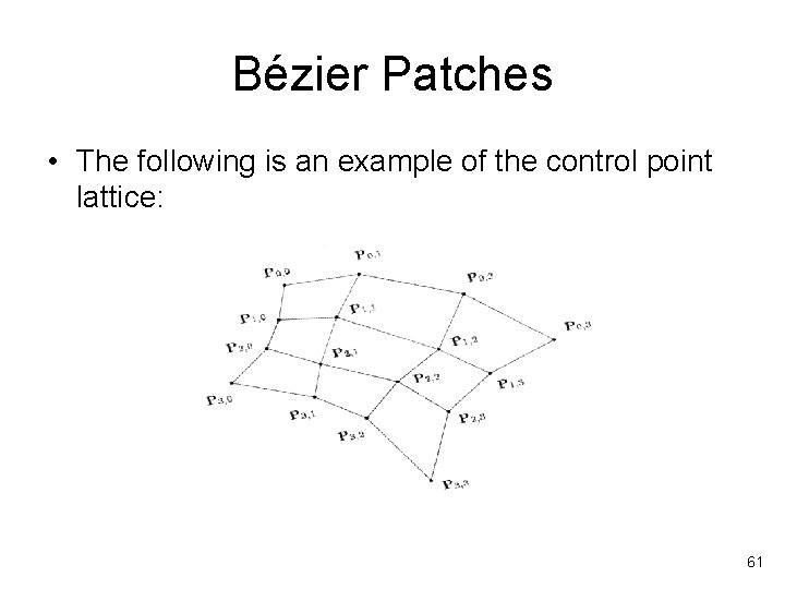
Bézier Patches • The following is an example of the control point lattice: 61

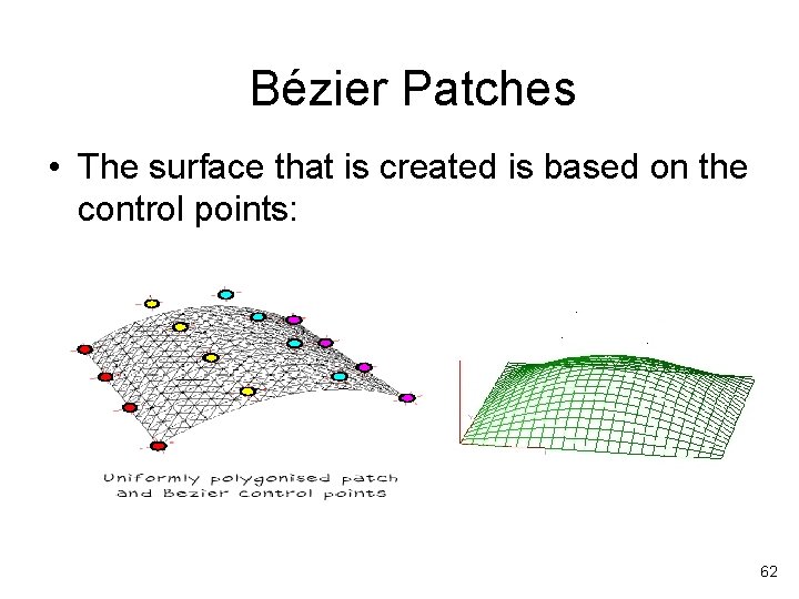
Bézier Patches • The surface that is created is based on the control points: 62

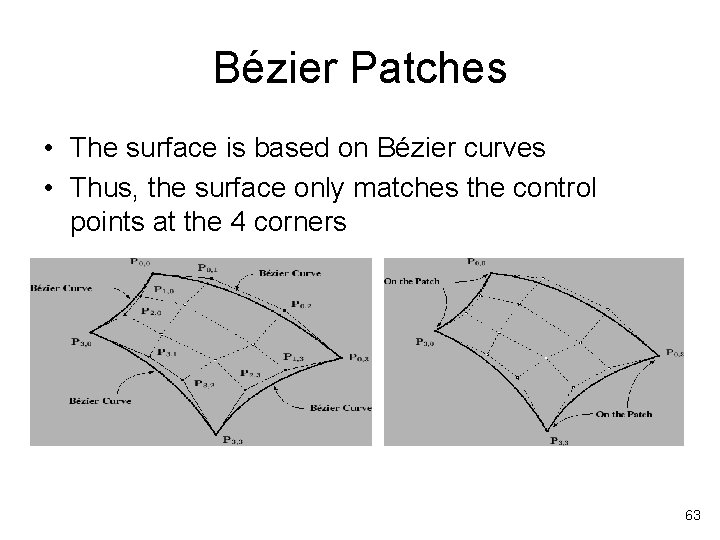
Bézier Patches • The surface is based on Bézier curves • Thus, the surface only matches the control points at the 4 corners 63

Bézier Patches • Adjusting the control points changes the shape of the surface: • See the applet on: – http: //www. nbb. cornell. edu/neurobio/land/Old. Student. Projects/cs 490 -96 to 97/anson/Bezier. Patch. Applet/ • All the same issue occur with patches as with curves – Control points have global control – Increasing the number of control points will increase the degree of the patch 64

Bézier Patches • Thus, we handle large curvy surfaces the same was as with curves: join patches together • Recall the continuity constrains: – C 0 continuity: edges must match – C 1 continuity: colinear control points • More difficult near joins of 4 patches 65

B-Spline Patches • B-Spline patches are similar to Bézier patches except that they are based on BSpline curves • This implies that: – You can have any number of control points in either the u or v direction (4 x 4, 8 x 12, etc. ) and still maintain piecewise C 2 cubic patches – With Uniform patches, the patch is will no go through the control points • See P. 116 in Games book 66

Rendering Patches • There are two types of ways we can render patches: – Render them directly from the parametric descriptions in hardware • Must have hardware support – Approximate the patch with a triangle mesh and render this mesh • Usually done in software • Standard pipeline can be used 67

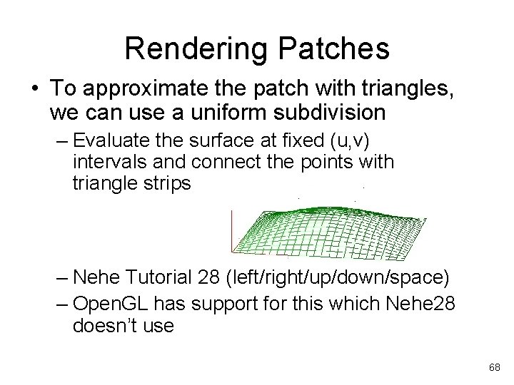
Rendering Patches • To approximate the patch with triangles, we can use a uniform subdivision – Evaluate the surface at fixed (u, v) intervals and connect the points with triangle strips – Nehe Tutorial 28 (left/right/up/down/space) – Open. GL has support for this which Nehe 28 doesn’t use 68

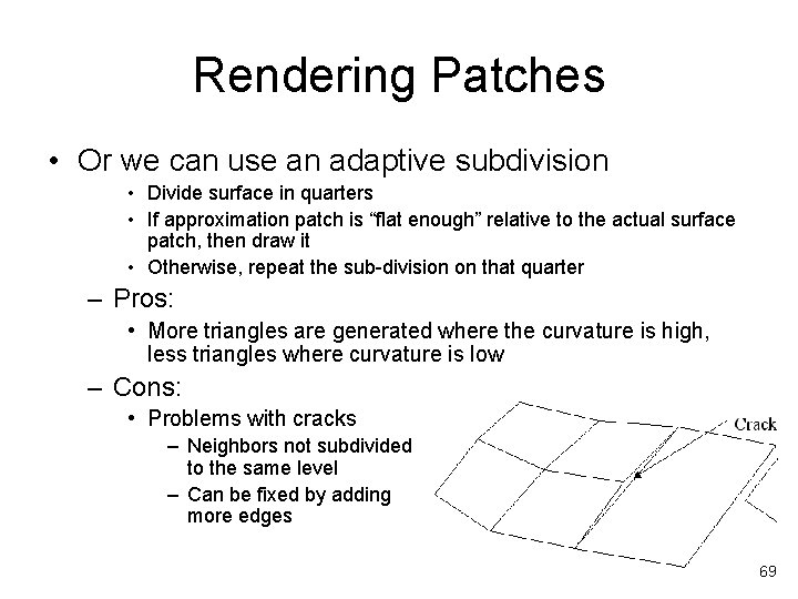
Rendering Patches • Or we can use an adaptive subdivision • Divide surface in quarters • If approximation patch is “flat enough” relative to the actual surface patch, then draw it • Otherwise, repeat the sub-division on that quarter – Pros: • More triangles are generated where the curvature is high, less triangles where curvature is low – Cons: • Problems with cracks – Neighbors not subdivided to the same level – Can be fixed by adding more edges 69

Rendering Patches • To have proper lighting we also need normals for the triangles – We can simply use the triangles normal – Or, if we want to be more accurate, we can use the actual normal to the parametric surface • Partial derivative in the u direction is 1 st tangent • Partial derivative in the v direction is 2 nd tangent • Take their cross product and normalize to produce the normal vector 70

Open. GL Bézier Curve Support • To setup a Bézier curve: – gl. Map 1 f(GL_MAP 1_VERTEX_3, 0. 0, 1. 0, 3, 4, &control. Pts[0][0]); • Params are: map type, u start, u end, stride, order (degree + 1), array of control points – gl. Enable(GL_MAP 1_VERTEX_3); • To setup a grid for subdivision – gl. Map. Grid 1 f(100, 0. 0, 10. 0) • 100 subdivision between starting with 0 and ending with 10 • Grid 0 gets mapped to u=0, grid 10 get mapped to u=1 • To draw the curve – gl. Eval. Mesh 1(GL_LINE, 0, 10) • Draw lines to approximate the curve from grid range 0 to 10 71

Open. GL Bézier Patch Support – gl. Map 2 f(GL_MAP 2_VERTEX_3, 0. 0, 1. 0, 3, 4, 0. 0, 12, 4, &control. Pts[0][0][0]); – gl. Enable(GL_MAP 2_VERTEX_3); – gl. Map. Grid 2 f(100, 0. 0 f, 10. 0 f); – gl. Eval. Mesh 2(GL_LINE, 0, 10); • Or GL_FILL which produces lit, shaded surface if lighting is turned on and we have normals for our surface – gl. Enable(GL_AUTO_NORMAL); • Texture mapping can also be done by using similar mapping to automatically generate texture coordinates 72

Open. GL NURBS Support • To setup the NURBS: – GLUnurbs. Obj *my. Nurb = glu. New. Nurbs. Renderer(); – glu. Nurbs. Property(my. Nurb, GLU_SAMPLING_TOLERANCE, max. Unit. Length); – glu. Nurbs. Property(my. Nurb, GLU_DISPLAY_MODE, GLU_FILL); • To display the NURBS: – glu. Begin. Surface(my. Nurb); – glu. Nurbs. Surface(my. Nurb, u. Knot. Count, u. Knot. Array, v. Knot. Count, v. Knot. Array, u. Stride, v. Stride, control. Pts. Array, u. Order, v. Order, GL_MAP 2_VERTEX_3); – glu. End. Surface(my. Nurb); • Tons more parameters and control available 73