Chapter 6 Scatterplots Association and Correlation Copyright 2015

Chapter 6 Scatterplots, Association and Correlation Copyright © 2015, 2010, 2007 Pearson Education, Inc. Chapter 6, Slide 1 -11

Looking at Scatterplots n n Scatterplots may be the most common and most effective display for data. n In a scatterplot, you can see patterns, trends, relationships, and even the occasional extraordinary value sitting apart from the others. Scatterplots are the best way to start observing the relationship and the ideal way to picture associations between two quantitative variables. Copyright © 2015, 2010, 2007 Pearson Education, Inc. Chapter 6, Slide 1 -22

Looking at Scatterplots (cont. ) n n When looking at scatterplots, we will find the direction, form, strength, and unusual features. When asked about the “association” in a scatterplot, this is what you write about! Copyright © 2015, 2010, 2007 Pearson Education, Inc. Chapter 6, Slide 1 -33

Direction n n A pattern that runs from the upper left to the lower right is said to have a negative direction. A trend running the other way has a positive direction Copyright © 2015, 2010, 2007 Pearson Education, Inc. Chapter 6, Slide 1 -44

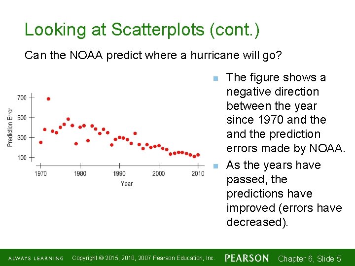
Looking at Scatterplots (cont. ) Can the NOAA predict where a hurricane will go? n n Copyright © 2015, 2010, 2007 Pearson Education, Inc. The figure shows a negative direction between the year since 1970 and the prediction errors made by NOAA. As the years have passed, the predictions have improved (errors have decreased). Chapter 6, Slide 1 -55

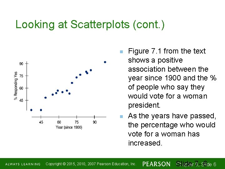
Looking at Scatterplots (cont. ) n n Figure 7. 1 from the text shows a positive association between the year since 1900 and the % of people who say they would vote for a woman president. As the years have passed, the percentage who would vote for a woman has increased. Copyright © 2015, 2010, 2007 Pearson Education, Inc. Chapter 76, Slide 61 -66

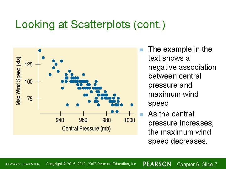
Looking at Scatterplots (cont. ) n n Copyright © 2015, 2010, 2007 Pearson Education, Inc. The example in the text shows a negative association between central pressure and maximum wind speed As the central pressure increases, the maximum wind speed decreases. Chapter 6, Slide 1 -77

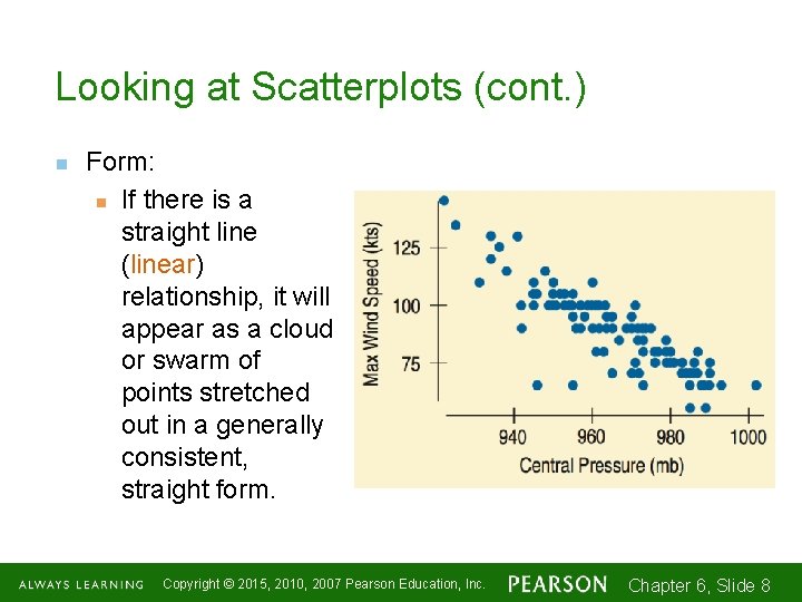
Looking at Scatterplots (cont. ) n Form: n If there is a straight line (linear) relationship, it will appear as a cloud or swarm of points stretched out in a generally consistent, straight form. Copyright © 2015, 2010, 2007 Pearson Education, Inc. Chapter 6, Slide 1 -88

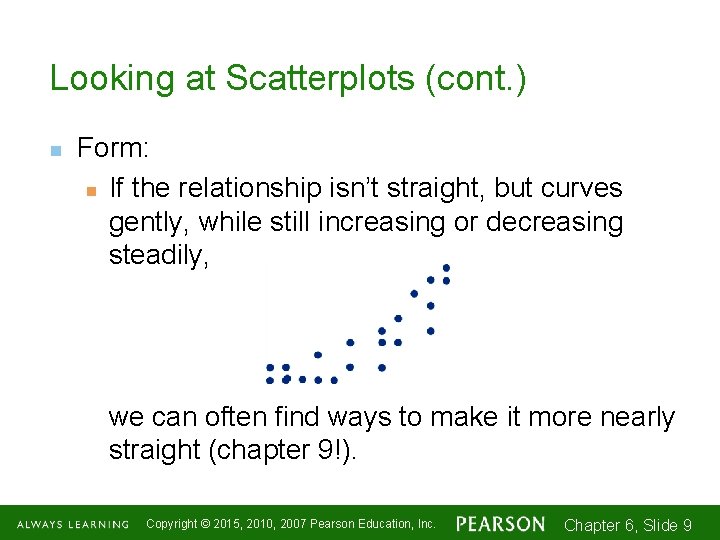
Looking at Scatterplots (cont. ) n Form: n If the relationship isn’t straight, but curves gently, while still increasing or decreasing steadily, we can often find ways to make it more nearly straight (chapter 9!). Copyright © 2015, 2010, 2007 Pearson Education, Inc. Chapter 6, Slide 1 -99

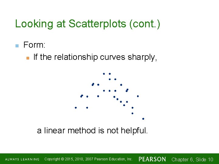
Looking at Scatterplots (cont. ) n Form: n If the relationship curves sharply, a linear method is not helpful. Copyright © 2015, 2010, 2007 Pearson Education, Inc. Chapter 6, Slide 1 -1010

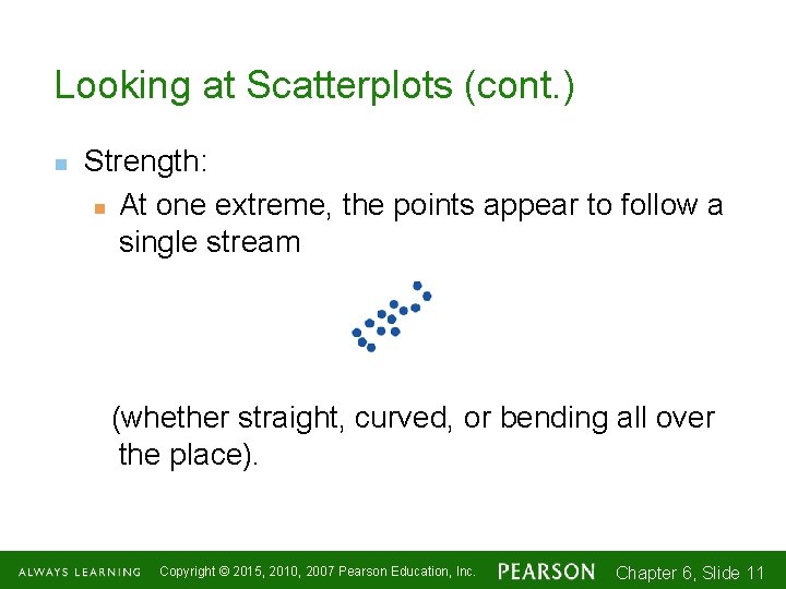
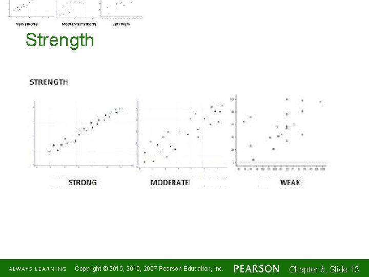
Looking at Scatterplots (cont. ) n Strength: n At one extreme, the points appear to follow a single stream (whether straight, curved, or bending all over the place). Copyright © 2015, 2010, 2007 Pearson Education, Inc. Chapter 6, Slide 1 -1111

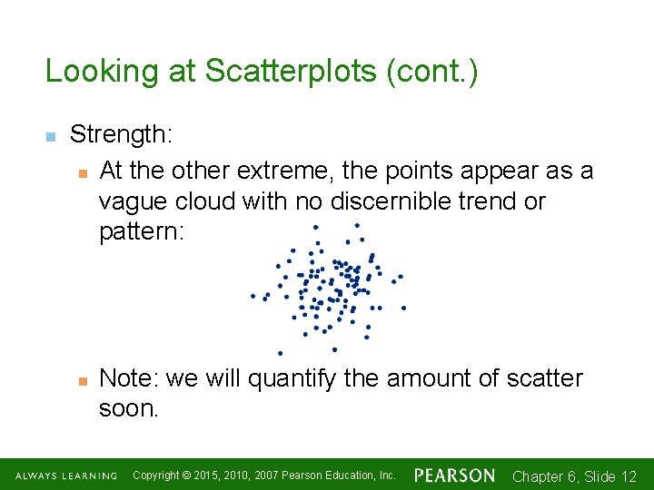
Looking at Scatterplots (cont. ) n Strength: n At the other extreme, the points appear as a vague cloud with no discernible trend or pattern: n Note: we will quantify the amount of scatter soon. Copyright © 2015, 2010, 2007 Pearson Education, Inc. Chapter 6, Slide 1 -1212

Strength Copyright © 2015, 2010, 2007 Pearson Education, Inc. Chapter 6, Slide 1 -1313

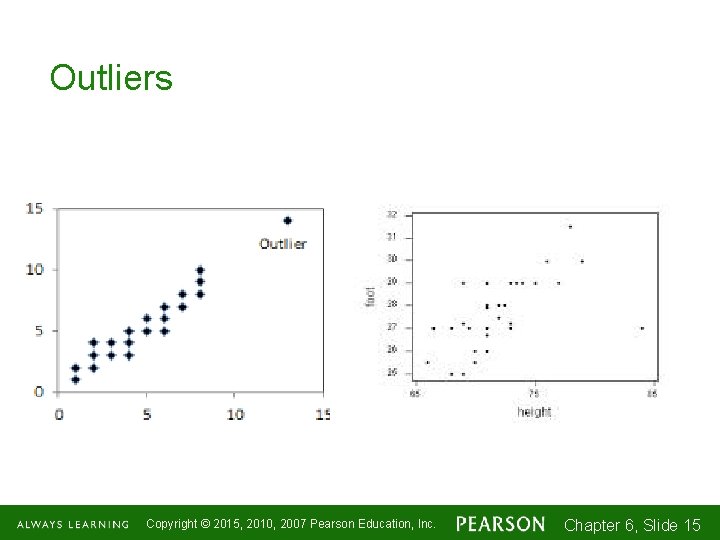
Looking at Scatterplots (cont. ) n Unusual features: n Look for the unexpected. n Often the most interesting thing to see in a scatterplot is the thing you never thought to look for. n One example of such a surprise is an outlier standing away from the overall pattern of the scatterplot. n Clusters or subgroups should also raise questions. Copyright © 2015, 2010, 2007 Pearson Education, Inc. Chapter 6, Slide 1 -1414

Outliers Copyright © 2015, 2010, 2007 Pearson Education, Inc. Chapter 6, Slide 1 -1515

Roles for Variables n n n It is important to determine which of the two quantitative variables goes on the x-axis and which on the y-axis. This determination is made based on the roles played by the variables. When the roles are clear, the explanatory or predictor variable goes on the x-axis, and the response variable (variable of interest) goes on the y-axis. Copyright © 2015, 2010, 2007 Pearson Education, Inc. Chapter 6, Slide 1 -1616

Roles for Variables (cont. ) n n The roles that we choose for variables are more about how we think about them rather than about the variables themselves. Just placing a variable on the x-axis doesn’t necessarily mean that it explains or predicts anything. And the variable on the y-axis may not respond to it in any way. Copyright © 2015, 2010, 2007 Pearson Education, Inc. Chapter 6, Slide 1 -1717

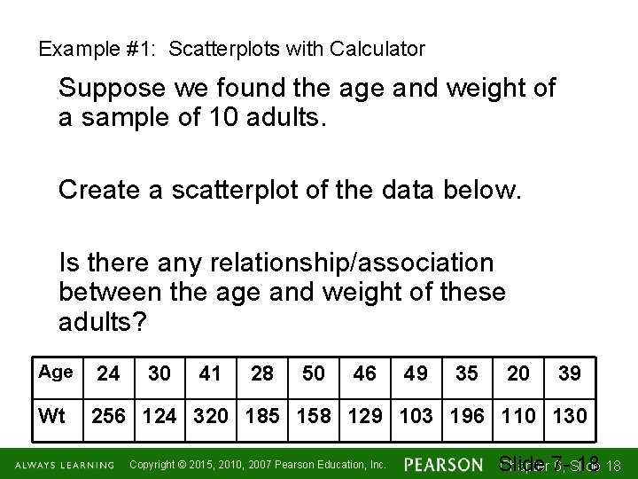
Example #1: Scatterplots with Calculator Suppose we found the age and weight of a sample of 10 adults. Create a scatterplot of the data below. Is there any relationship/association between the age and weight of these adults? Age Wt 24 30 41 28 50 46 49 35 20 39 256 124 320 185 158 129 103 196 110 130 Copyright © 2015, 2010, 2007 Pearson Education, Inc. Chapter 76, Slide 18 1 -1818

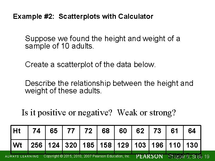
Example #2: Scatterplots with Calculator Suppose we found the height and weight of a sample of 10 adults. Create a scatterplot of the data below. Describe the relationship between the height and weight of these adults. Is it positive or negative? Weak or strong? Ht 74 65 77 72 68 60 Wt 256 124 320 185 158 129 103 196 110 130 Copyright © 2015, 2010, 2007 Pearson Education, Inc. 62 73 61 64 Chapter 76, Slide 19 1 -1919

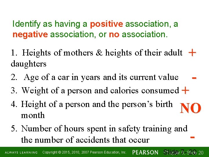
Identify as having a positive association, a negative association, or no association. 1. Heights of mothers & heights of their adult + daughters 2. Age of a car in years and its current value 3. Weight of a person and calories consumed + 4. Height of a person and the person’s birth NO month 5. Number of hours spent in safety training and the number of accidents that occur Copyright © 2015, 2010, 2007 Pearson Education, Inc. Chapter 76, Slide 20 1 -2020

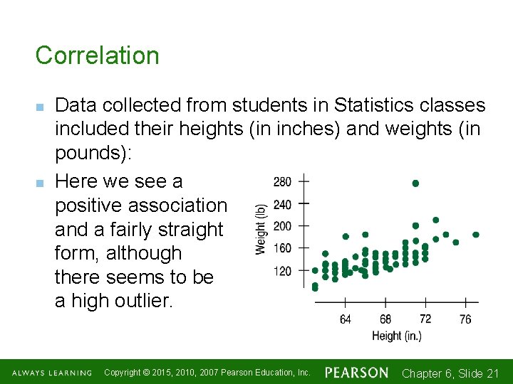
Correlation n n Data collected from students in Statistics classes included their heights (in inches) and weights (in pounds): Here we see a positive association and a fairly straight form, although there seems to be a high outlier. Copyright © 2015, 2010, 2007 Pearson Education, Inc. Chapter 6, Slide 1 -2121

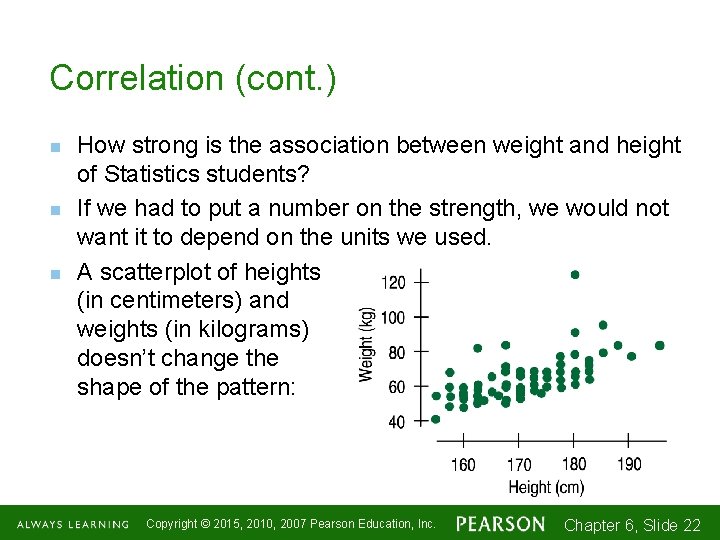
Correlation (cont. ) n n n How strong is the association between weight and height of Statistics students? If we had to put a number on the strength, we would not want it to depend on the units we used. A scatterplot of heights (in centimeters) and weights (in kilograms) doesn’t change the shape of the pattern: Copyright © 2015, 2010, 2007 Pearson Education, Inc. Chapter 6, Slide 1 -2222

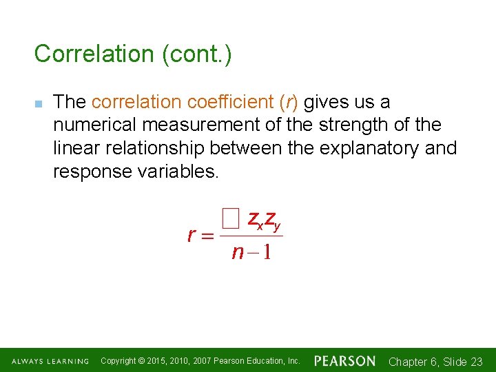
Correlation (cont. ) n The correlation coefficient (r) gives us a numerical measurement of the strength of the linear relationship between the explanatory and response variables. Copyright © 2015, 2010, 2007 Pearson Education, Inc. Chapter 6, Slide 1 -2323

Properties of r (correlation coefficient) n legitimate values of r is [-1, 1] No Correlation Strong correlation Moderate Correlation Weak correlation Copyright © 2015, 2010, 2007 Pearson Education, Inc. Chapter 76, Slide 24 1 -2424

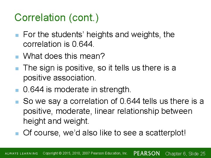
Correlation (cont. ) n n n For the students’ heights and weights, the correlation is 0. 644. What does this mean? The sign is positive, so it tells us there is a positive association. 0. 644 is moderate in strength. So we say a correlation of 0. 644 tells us there is a positive, moderate, linear relationship between height and weight. Of course, we’d also like to see a scatterplot! Copyright © 2015, 2010, 2007 Pearson Education, Inc. Chapter 6, Slide 1 -2525

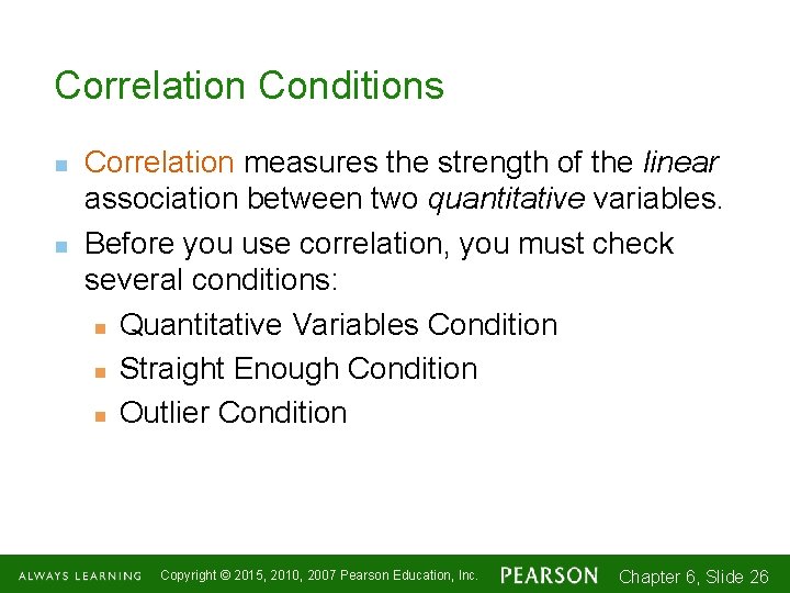
Correlation Conditions n n Correlation measures the strength of the linear association between two quantitative variables. Before you use correlation, you must check several conditions: n Quantitative Variables Condition n Straight Enough Condition n Outlier Condition Copyright © 2015, 2010, 2007 Pearson Education, Inc. Chapter 6, Slide 1 -2626

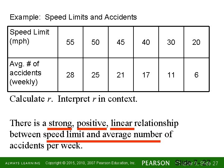
Example: Speed Limits and Accidents Speed Limit (mph) Avg. # of accidents (weekly) 55 50 45 40 30 20 28 25 21 17 11 6 Calculate r. Interpret r in context. There is a strong, positive, linear relationship between speed limit and average number of accidents per week. Copyright © 2015, 2010, 2007 Pearson Education, Inc. Chapter 76, Slide 27 1 -2727

Homework: n Page 164: 3, 4, 5, 11, 14, 17, 34 n Reading Chapter 7 (yellow textbook) n Interpreting Center & Variability Worksheet n Indian Tribe Extra Credit (Optional) Copyright © 2015, 2010, 2007 Pearson Education, Inc. Chapter 6, Slide 1 -2828

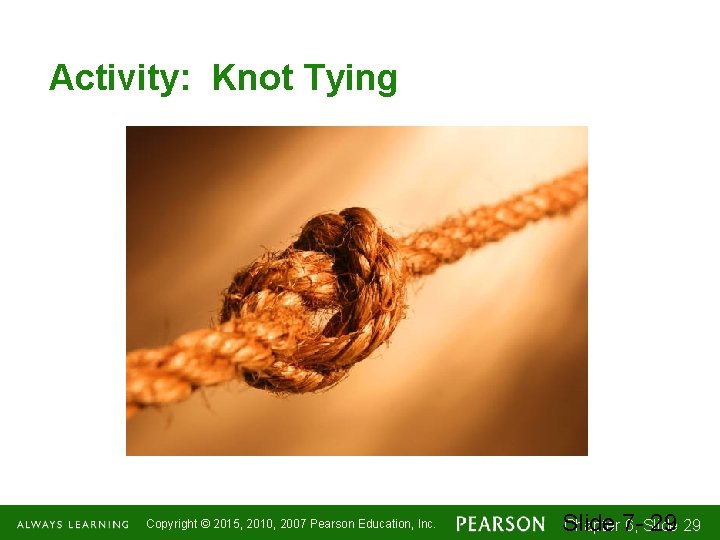
Activity: Knot Tying Copyright © 2015, 2010, 2007 Pearson Education, Inc. Chapter 76, Slide 29 1 -2929

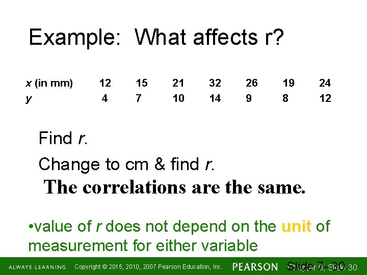
Example: What affects r? x (in mm) y 12 4 15 7 21 10 32 14 26 9 19 8 24 12 Find r. Change to cm & find r. The correlations are the same. • value of r does not depend on the unit of measurement for either variable Copyright © 2015, 2010, 2007 Pearson Education, Inc. Chapter 76, Slide 30 1 -3030

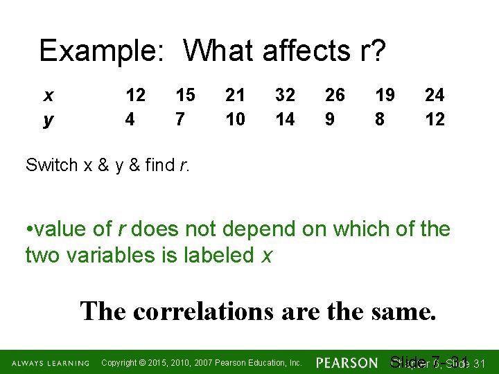
Example: What affects r? x y 12 4 15 7 21 10 32 14 26 9 19 8 24 12 Switch x & y & find r. • value of r does not depend on which of the two variables is labeled x The correlations are the same. Copyright © 2015, 2010, 2007 Pearson Education, Inc. Chapter 76, Slide 31 1 -3131

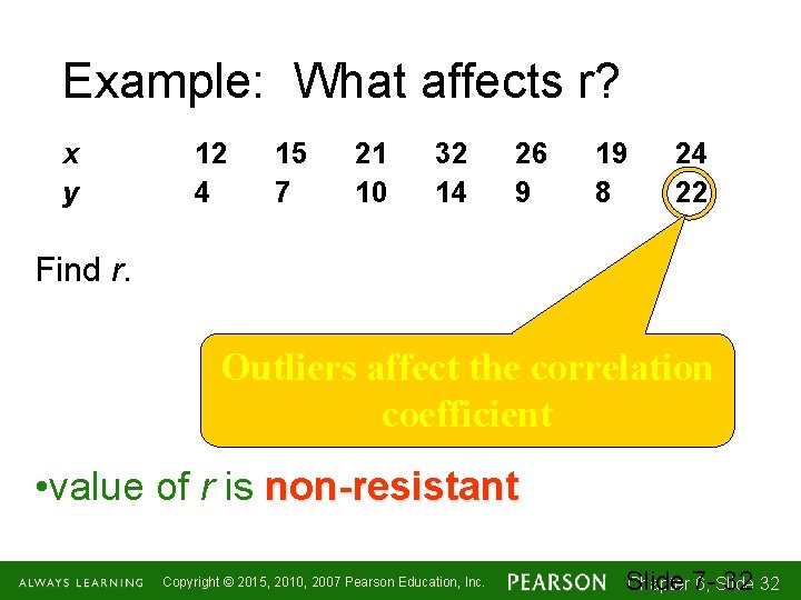
Example: What affects r? x y 12 4 15 7 21 10 32 14 26 9 19 8 24 22 Find r. Outliers affect the correlation coefficient • value of r is non-resistant Copyright © 2015, 2010, 2007 Pearson Education, Inc. Chapter 76, Slide 32 1 -3232

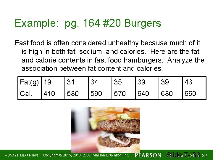
Example: pg. 164 #20 Burgers Fast food is often considered unhealthy because much of it is high in both fat, sodium, and calories. Here are the fat and calorie contents in fast food hamburgers. Analyze the association between fat content and calories. Fat(g) 19 31 34 35 39 39 43 Cal. 580 590 570 640 680 660 410 Copyright © 2015, 2010, 2007 Pearson Education, Inc. Chapter 76, Slide 33 1 -3333

Correlation Conditions (cont. ) n Quantitative Variables Condition: n Correlation applies only to quantitative variables. n Don’t apply correlation to categorical data masquerading as quantitative. n Check that you know the variables’ units and what they measure. Copyright © 2015, 2010, 2007 Pearson Education, Inc. Chapter 6, Slide 1 -3434

Correlation Conditions (cont. ) n Straight Enough Condition: n Correlation measures the strength only of the linear association, and will be misleading if the relationship is not linear. n Thus we only calculate and use the correlation coefficient for linear data. Copyright © 2015, 2010, 2007 Pearson Education, Inc. Chapter 6, Slide 1 -3535

Correlation Conditions (cont. ) n Outlier Condition: n Outliers can distort the correlation dramatically. n An outlier can make an otherwise small correlation look big or hide a large correlation. n It can even give an otherwise positive association a negative correlation coefficient (and vice versa). n When you see an outlier, it’s often a good idea to report the correlations with and without the point. Copyright © 2015, 2010, 2007 Pearson Education, Inc. Chapter 6, Slide 1 -3636

Correlation Properties n n The sign of a correlation coefficient gives the direction of the association. Correlation is always between – 1 and +1. n Correlation can be exactly equal to – 1 or +1, but these values are unusual in real data because they mean that all the data points fall exactly on a single straight line. n A correlation near zero corresponds to a weak linear association. Copyright © 2015, 2010, 2007 Pearson Education, Inc. Chapter 6, Slide 1 -3737

Correlation Properties (cont. ) n n n Correlation treats x and y symmetrically: n The correlation of x with y is the same as the correlation of y with x. Correlation has no units. Correlation is not affected by changes in the center or scale of either variable. n Correlation depends only on the z-scores, and they are unaffected by changes in center or scale. Copyright © 2015, 2010, 2007 Pearson Education, Inc. Chapter 6, Slide 1 -3838

Correlation Properties (cont. ) n n Correlation measures the strength of the linear association between the two variables. n Variables can have a strong association but still have a small correlation if the association isn’t linear. Correlation is sensitive to outliers. A single outlying value can make a small correlation large or make a large one small. Copyright © 2015, 2010, 2007 Pearson Education, Inc. Chapter 6, Slide 1 -3939

Review Question! n n Which statistics have we studied so far this year that are resistant? Which statistics are not resistant? Copyright © 2015, 2010, 2007 Pearson Education, Inc. Chapter 6, Slide 1 -4040

Correlation does not imply causation Copyright © 2015, 2010, 2007 Pearson Education, Inc. Chapter 76, Slide 41 1 -4141

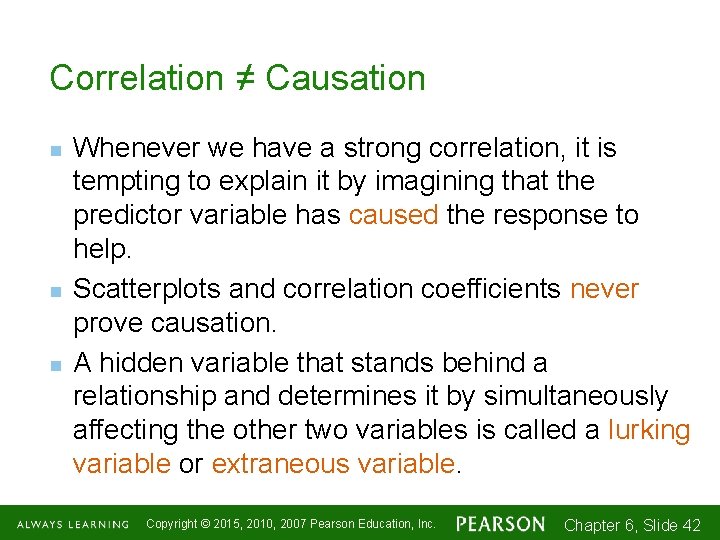
Correlation ≠ Causation n Whenever we have a strong correlation, it is tempting to explain it by imagining that the predictor variable has caused the response to help. Scatterplots and correlation coefficients never prove causation. A hidden variable that stands behind a relationship and determines it by simultaneously affecting the other two variables is called a lurking variable or extraneous variable. Copyright © 2015, 2010, 2007 Pearson Education, Inc. Chapter 6, Slide 1 -4242

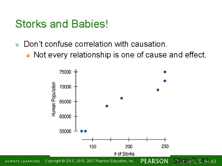
Storks and Babies! n Don’t confuse correlation with causation. n Not every relationship is one of cause and effect. Copyright © 2015, 2010, 2007 Pearson Education, Inc. Chapter 76, Slide 43 1 -4343

Example: Association vs. Causation – Methodist Ministers and Rum Look at the table in your outline. What is the correlation? What does this mean? Is there a lurking variable? Copyright © 2015, 2010, 2007 Pearson Education, Inc. Chapter 76, Slide 44 1 -4444

Straightening Scatterplots n n n Straight line relationships are the ones that we can measure with correlation. When a scatterplot shows a bent form that consistently increases or decreases, we can often straighten the form of the plot by re-expressing one or both variables. We will cover straightening techniques in Chapter 9. Copyright © 2015, 2010, 2007 Pearson Education, Inc. Chapter 6, Slide 1 -4545

What Can Go Wrong? n Don’t say “correlation” when you mean “association. ” n More often than not, people say correlation when they mean association. n The word “correlation” should be reserved for measuring the strength and direction of the linear relationship between two quantitative variables. Copyright © 2015, 2010, 2007 Pearson Education, Inc. Chapter 6, Slide 1 -4646

What Can Go Wrong? n n Don’t correlate categorical variables. n Be sure to check the Quantitative Variables Condition. Don’t confuse “correlation” with “causation. ” n Scatterplots and correlations never demonstrate causation. n These statistical tools can only demonstrate an association between variables. Copyright © 2015, 2010, 2007 Pearson Education, Inc. Chapter 6, Slide 1 -4747

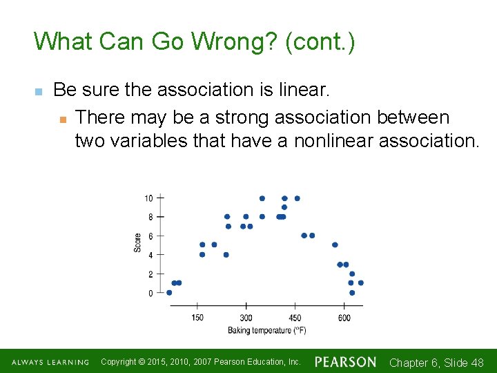
What Can Go Wrong? (cont. ) n Be sure the association is linear. n There may be a strong association between two variables that have a nonlinear association. Copyright © 2015, 2010, 2007 Pearson Education, Inc. Chapter 6, Slide 1 -4848

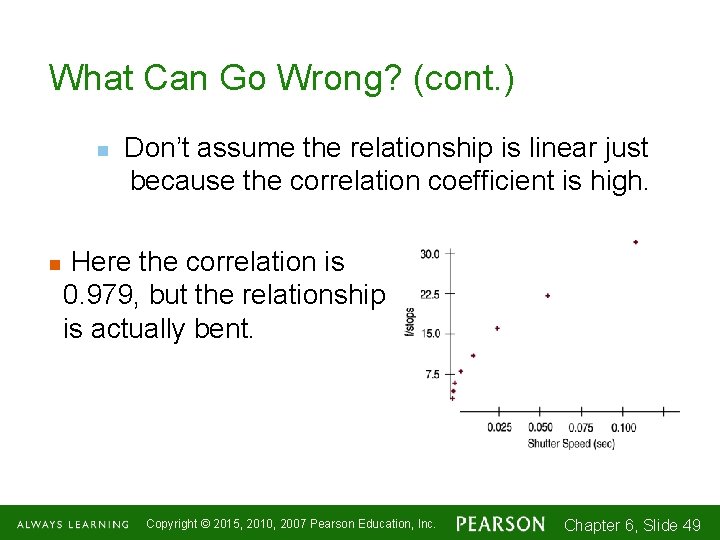
What Can Go Wrong? (cont. ) n n Don’t assume the relationship is linear just because the correlation coefficient is high. Here the correlation is 0. 979, but the relationship is actually bent. Copyright © 2015, 2010, 2007 Pearson Education, Inc. Chapter 6, Slide 1 -4949

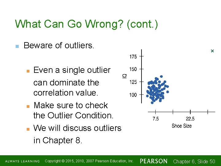
What Can Go Wrong? (cont. ) n Beware of outliers. n n n Even a single outlier can dominate the correlation value. Make sure to check the Outlier Condition. We will discuss outliers in Chapter 8. Copyright © 2015, 2010, 2007 Pearson Education, Inc. Chapter 6, Slide 1 -5050

What have we learned? n n We examine scatterplots for direction, form, strength, and unusual features. Although not every relationship is linear, when the scatterplot is straight enough, the correlation coefficient is a useful numerical summary. n The sign of the correlation tells us the direction of the association. n The magnitude of the correlation tells us the strength of a linear association. n Correlation has no units, so shifting or scaling the data, standardizing, or swapping the variables has no effect on the numerical value. Copyright © 2015, 2010, 2007 Pearson Education, Inc. Chapter 6, Slide 1 -5151

What have we learned? (cont. ) n n Doing Statistics right means that we have to Think about whether our choice of methods is appropriate. n Before finding or talking about a correlation, check the Straight Enough Condition. n Watch out for outliers! Don’t assume that a high correlation or strong association is evidence of a cause-and-effect relationship—beware of lurking variables! Copyright © 2015, 2010, 2007 Pearson Education, Inc. Chapter 6, Slide 1 -5252

AP Tips n n n Just like the rest of the graphs in this course, scales and labels are required for full credit. You don’t have to start either axes at zero, but once you start scaling an axes, it should keep the same scale for its entire length. Describing a scatterplot should be done in context and include the form, strength and association. n “There is a strong, positive, and linear relationship between age and height. ” Copyright © 2015, 2010, 2007 Pearson Education, Inc. Chapter 6, Slide 1 -5454

AP Tips, cont. n We usually refer to r as simply correlation. But the AP test usually refers to r as the correlation coefficient. Don’t get confused by the additional word coefficient. It’s just r. Copyright © 2015, 2010, 2007 Pearson Education, Inc. Chapter 6, Slide 1 -5555