Introduction to Bivariate Data and Scatterplots Regression 1

Bivariate Data � Most statistical studies involve more than one variable. � Suppose each individual in the sample provides two variable values. � Objective is to discover a relationship (or lack thereof) between the variables. ◦ Do some variables tend to vary together? ◦ Do some variables explain variability in another? response variable measures or records an outcome of a study. (Also: y, dependent variable, predicted variable) �A explanatory variable explains changes in the response variable. (Also: x, independent variable, predictor variable) � An

Finding Associations � � We can say two variables have an are association if knowing the value of one of the variables tells you something about the values of the other variable Simple examples ◦ Section at a Stadium and Price of ticket ◦ Stress level and lack of sleep � Types of data: ◦ Age and distance of commute (numerical vs. numerical) ◦ Is there is a difference in gender and cell phone provider (categorical vs. categorical) ◦ Height and favorite color (numerical vs. categorical) 3

Baseball’s Problem � In 1981, the average length of a game in Major League Baseball was 2 hours 33 minutes. Through 1, 054 games in 2014, that had jumped to a whopping 3 hours and 2 minutes. (Quote from Forbes Magazine). � MLB Leadership created a committee to study the length of Major League Baseball games. � The goals of the committee are to decrease the time of game and improve the overall pace of play

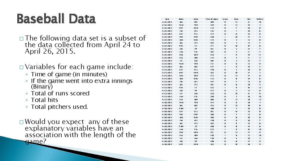
Baseball Data � The following data set is a subset of the data collected from April 24 to April 26, 2015. � Variables for each game include: ◦ Time of game (in minutes) ◦ If the game went into extra innings (Binary) ◦ Total of runs scored ◦ Total hits ◦ Total pitchers used. � Would you expect any of these explanatory variables have an association with the length of the game? Date Home Away Time of Game Extras Runs Hits Pitchers 4/24/2015 BAL BOS 209 0 12 21 10 4/24/2015 TAM TOR 149 0 15 19 5 4/24/2015 NYY NYM 153 0 7 16 6 4/24/2015 PHI ATL 154 0 1 10 6 4/24/2015 DET CLE 172 0 14 23 6 4/24/2015 CIN CHC 228 1 10 17 11 4/24/2015 MIA WAS 152 0 5 15 8 4/24/2015 MIL STL 162 0 3 13 7 4/24/2015 COL SF 171 0 10 27 8 4/24/2015 ARI PIT 161 0 5 14 7 4/24/2015 LAA TEX 167 0 5 11 7 4/24/2015 OAK HOU 216 1 9 19 11 4/24/2015 SEA MIN 123 0 2 11 2 4/24/2015 SD LAD 184 0 3 14 7 4/25/2015 TAM TOR 151 0 6 15 9 4/25/2015 BAL BOS 177 1 9 19 7 4/25/2015 DET CLE 178 0 5 16 8 4/25/2015 NYY NYM 165 0 10 17 5 4/25/2015 OAK HOU 175 0 12 17 6 4/25/2015 MIA WAS 155 0 8 19 6 4/25/2015 PHI ATL 147 0 7 15 8 4/25/2015 MIL STL 181 0 8 18 11 4/25/2015 COL SF 232 1 9 24 13 4/25/2015 ARI PIT 172 0 3 15 6 4/25/2015 SD LAD 216 0 19 21 9 4/25/2015 LAA TEX 190 0 5 16 10 4/25/2015 SEA MIN 206 0 13 18 12 4/26/2015 TAM TOR 143 0 6 18 5 4/26/2015 BAL BOS 193 0 25 29 8 4/26/2015 CHW KC 168 0 5 16 8 4/26/2015 DET CLE 181 0 14 23 8 4/26/2015 CIN CHC 166 0 7 12 8 4/26/2015 MIA WAS 160 0 8 18 8 4/26/2015 PHI ATL 158 0 9 16 7 4/26/2015 MIL STL 183 0 9 23 8 4/26/2015 CHW KC 168 0 8 14 8 4/26/2015 LAA TEX 253 1 9 24 10 4/26/2015 OAK HOU 191 0 13 17 9 4/26/2015 SEA MIN 220 1 6 15 10 4/26/2015 SD LAD 150 0 4 10 5 4/26/2015 ARI PIT 198 0 8 17 9 4/26/2015 NYY NYM 165 0 10 16 9

Examining Relationships Considering the relationship between two quantitative variables. � Start with a graph � Look for an overall pattern and deviations from the pattern � Use numerical descriptions of the data and overall pattern (if appropriate) � Consider a mathematical model (regression)

Scatterplots �A scatterplot is a graph displaying the relationship between two (typically quantitative) variables measured on the same set of individuals. � Typically we want: ◦ response variable on y-axis ◦ explanatory variable on x-axis � Each individual in the dataset appears as a point in the plot. 7

Baseball Data � Some potential Explanatory Variables with Time of game as the response: � What looks to be the “best” predictor? 8

Examining Relationships Considering the relationship between two quantitative variables. � Start with a graph � Look for an overall pattern (and potential deviations) � Use numerical descriptions of the data and overall pattern (if appropriate) � Consider a mathematical model (regression)

Interpreting Scatterplots � We describe the relationship between the two variables by examining the shape (or form), trend (or direction), and strength of the association. � We look for the overall pattern… ◦ Shape: linear, curved, clusters, no pattern ◦ Trend: positive, negative, no direction ◦ Strength: how closely the points fit the “shape” � Also, we will look for deviations (potential outliers) from the pattern. More on this later.

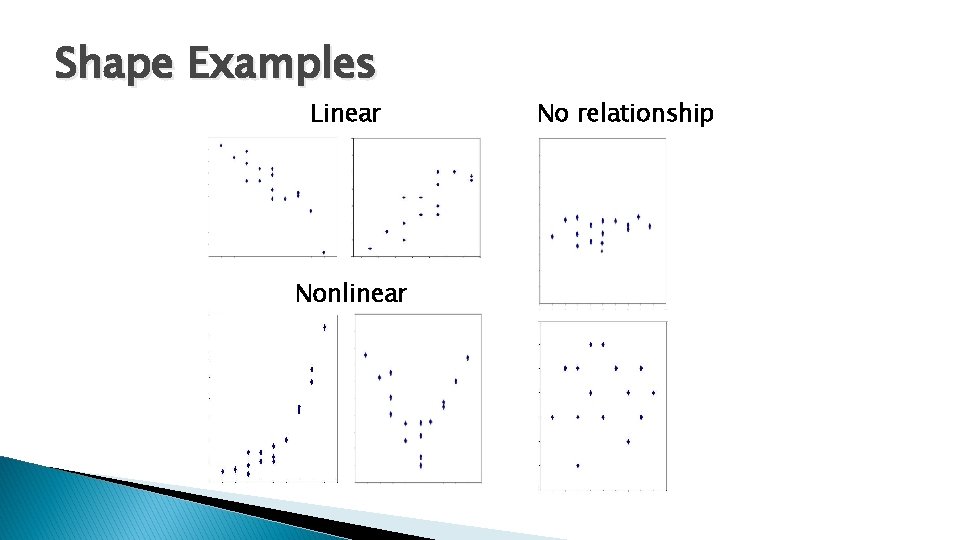
Shape Examples Linear Nonlinear No relationship

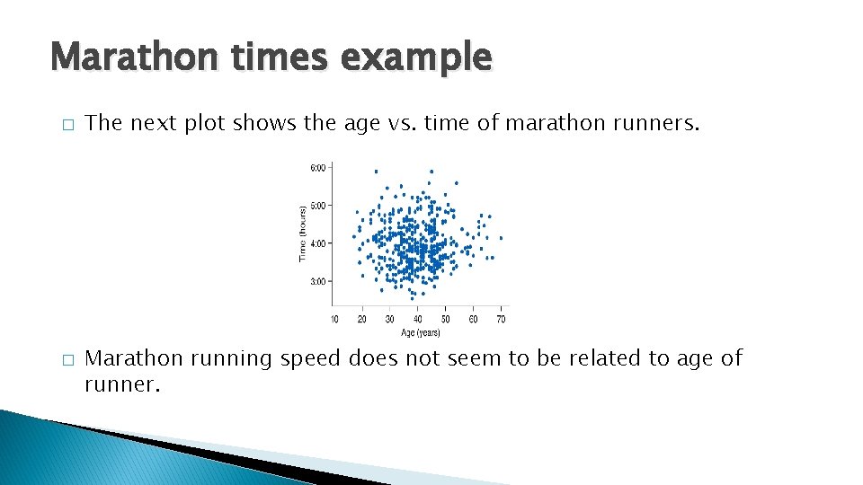
Marathon times example � � The next plot shows the age vs. time of marathon runners. Marathon running speed does not seem to be related to age of runner.

Notes on Shape � ALWAYS look at Shape first � For our purposes we will ONLY be able to work with Linear shapes. � There are methods that handle other shapes 13

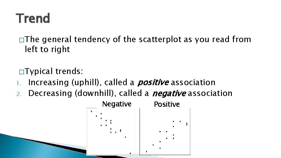
Trend � The general tendency of the scatterplot as you read from left to right � Typical 1. 2. trends: Increasing (uphill), called a positive association Decreasing (downhill), called a negative association Negative Positive

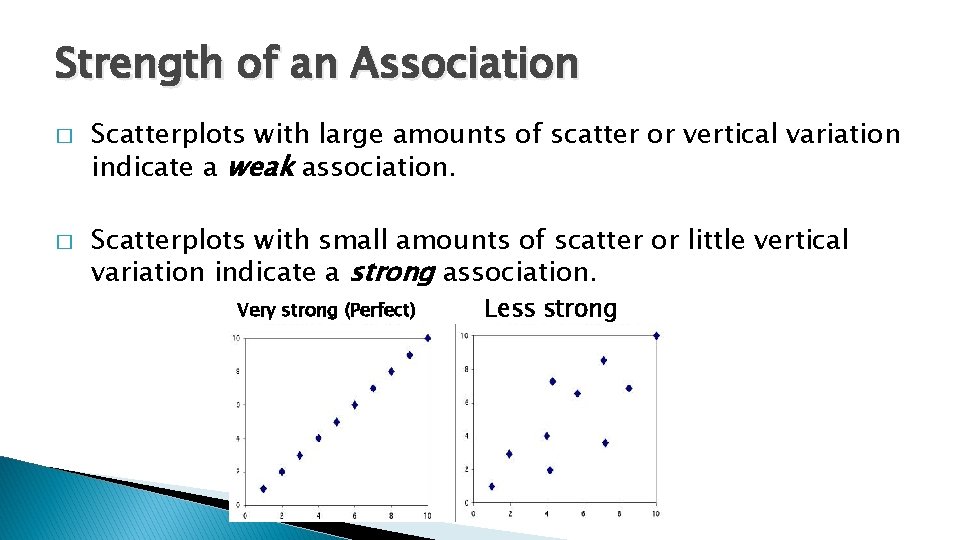
Strength of an Association � � Scatterplots with large amounts of scatter or vertical variation indicate a weak association. Scatterplots with small amounts of scatter or little vertical variation indicate a strong association. Very strong (Perfect) Less strong

Writing Descriptions of Associations � 1. 2. 3. � When writing a description of an association between two numerical variables, always include: Shape Trend Strength In addition, mention any observations that don’t fit the general trend (if any).

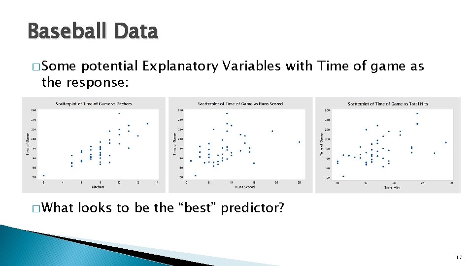
Baseball Data � Some potential Explanatory Variables with Time of game as the response: � What looks to be the “best” predictor? 17

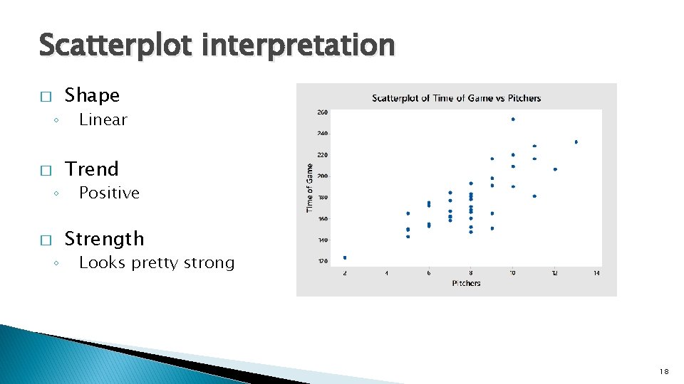
Scatterplot interpretation � ◦ � ◦ Shape Linear Trend Positive Strength Looks pretty strong 18

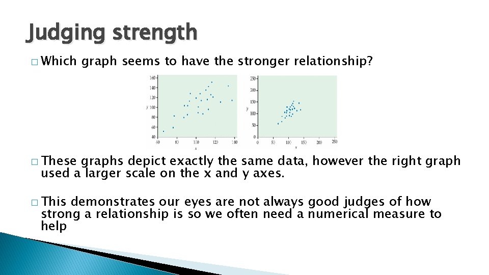
Judging strength � Which graph seems to have the stronger relationship? � These graphs depict exactly the same data, however the right graph used a larger scale on the x and y axes. � This demonstrates our eyes are not always good judges of how strong a relationship is so we often need a numerical measure to help

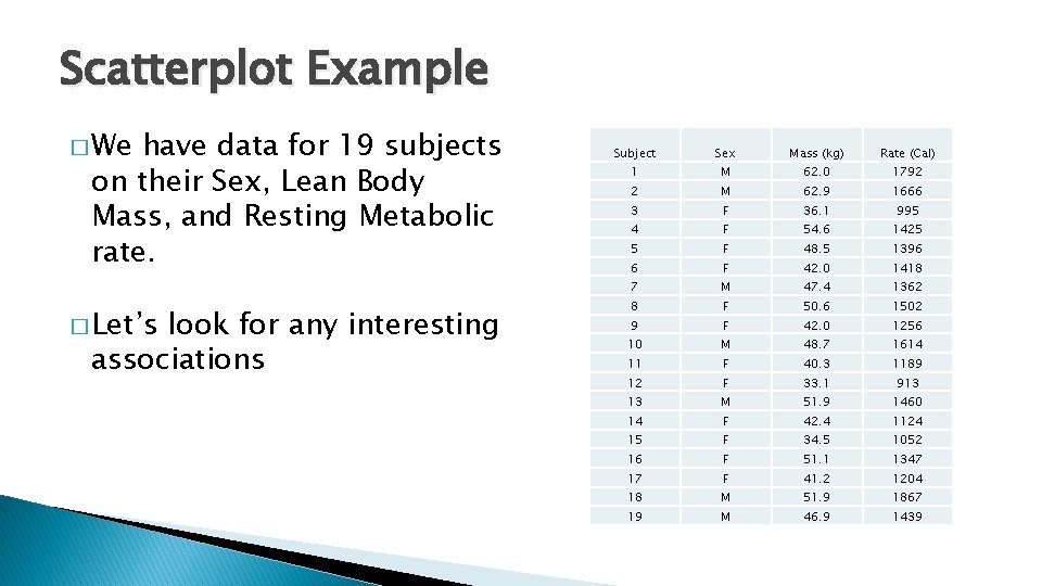
Scatterplot Example � We have data for 19 subjects on their Sex, Lean Body Mass, and Resting Metabolic rate. � Let’s look for any interesting associations Subject Sex Mass (kg) Rate (Cal) 1 M 62. 0 1792 2 M 62. 9 1666 3 F 36. 1 995 4 F 54. 6 1425 5 F 48. 5 1396 6 F 42. 0 1418 7 M 47. 4 1362 8 F 50. 6 1502 9 F 42. 0 1256 10 M 48. 7 1614 11 F 40. 3 1189 12 F 33. 1 913 13 M 51. 9 1460 14 F 42. 4 1124 15 F 34. 5 1052 16 F 51. 1 1347 17 F 41. 2 1204 18 M 51. 9 1867 19 M 46. 9 1439

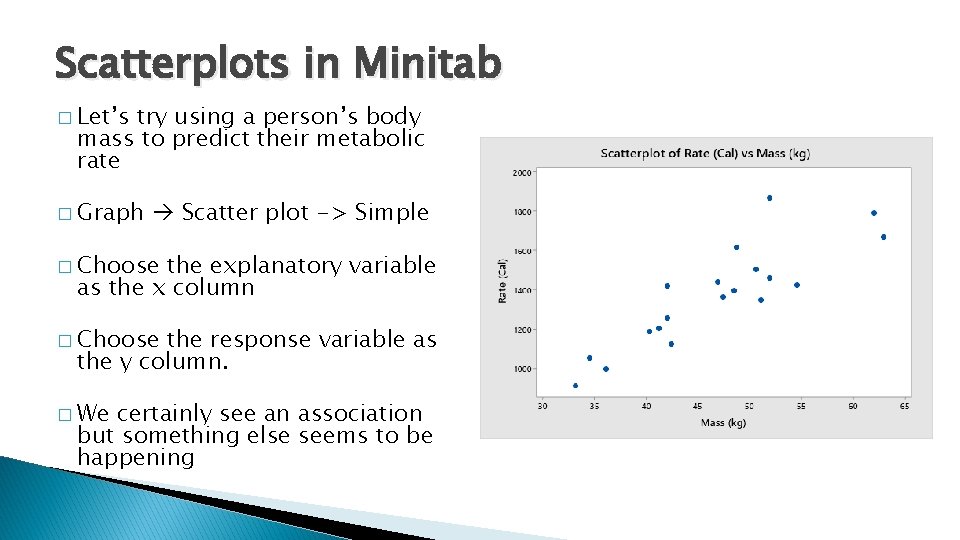
Scatterplots in Minitab � Let’s try using a person’s body mass to predict their metabolic rate � Graph Scatter plot -> Simple � Choose the explanatory variable as the x column � Choose the response variable as the y column. � We certainly see an association but something else seems to be happening

Categorical variables in Scatterplots � Recall the data types of on our 19 subjects: ◦ Lean Body Mass - Quantitative ◦ Resting Metabolic rate – Quantitative ◦ Sex - Categorical � Maybe � We there is a difference in associations between genders? could: ◦ Break the data up into two scatterplots ◦ View both genders in one plot

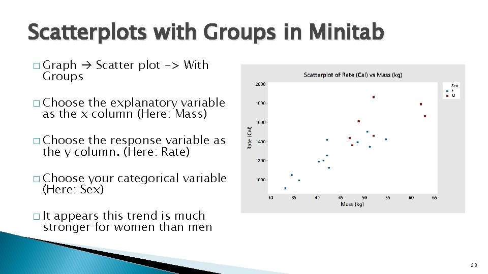
Scatterplots with Groups in Minitab � Graph Scatter plot -> With Groups � Choose the explanatory variable as the x column (Here: Mass) � Choose the response variable as the y column. (Here: Rate) � Choose your categorical variable (Here: Sex) � It appears this trend is much stronger for women than men 23