Automatic Speech Recognition Foundations in Language Science and

Automatic Speech Recognition Foundations in Language Science and Technology WS 2007 -8 FR 4. 7 Allgemeine Linguistik Institut für Phonetik, Ud. S (IPUS)

Overview • Variation in the realisation of words – phonological – phonetic • Modelling the acoustic Signal • Hidden-Markov-Modelling

Speech Recognition: Applications • Registration/Security identificaton systems (e. g. , Banking) • Enquiry systems (railway timetables) • Hands-free telephones • Speech Input to, e. g. navigation-systems • Aids for the handicapped • Dictation systems, e. g. Naturally. Speaking (Dragon/ Scansoft), Via. Voice (IBM), Free. Speech (Philips)

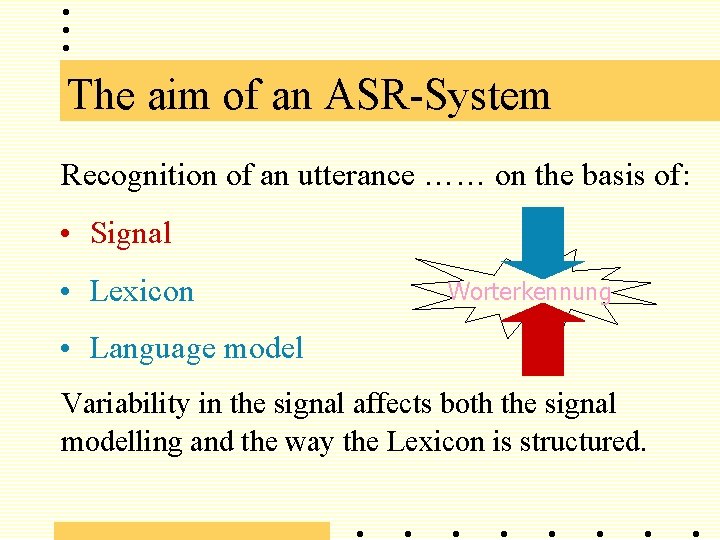
The aim of an ASR-System Recognition of an utterance …… on the basis of: • Signal • Lexicon Worterkennung • Language model Variability in the signal affects both the signal modelling and the way the Lexicon is structured.

Variation in the realisation of words Phonological and phonetic processes can result in different realisations of the same word: • Sound deletion • Epenthesis • Assimilation

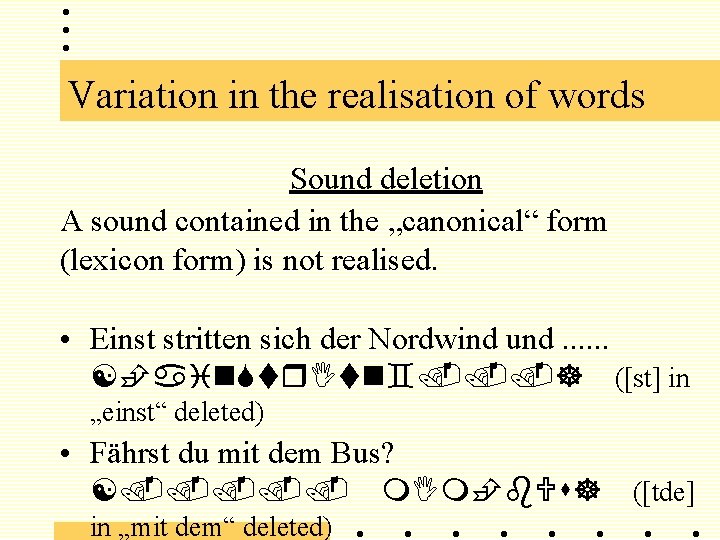
Variation in the realisation of words Sound deletion A sound contained in the „canonical“ form (lexicon form) is not realised. • Einst stritten sich der Nordwind und. . . ([st] in „einst“ deleted) • Fährst du mit dem Bus? . . . ([tde] in „mit dem“ deleted)

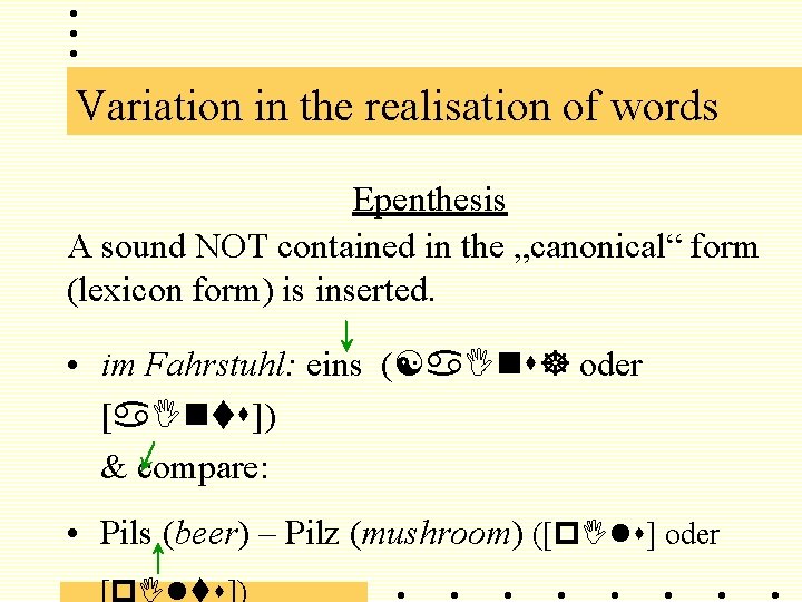
Variation in the realisation of words Epenthesis A sound NOT contained in the „canonical“ form (lexicon form) is inserted. • im Fahrstuhl: eins ( oder [ ]) & compare: • Pils (beer) – Pilz (mushroom) ([p l ] oder [p l ])

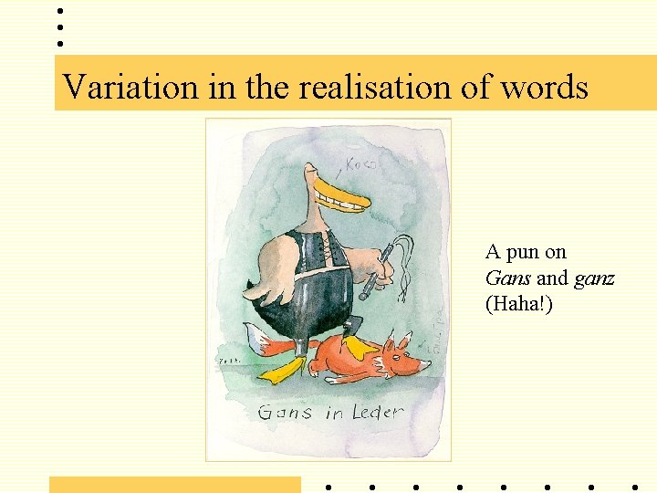
Variation in the realisation of words A pun on Gans and ganz (Haha!)

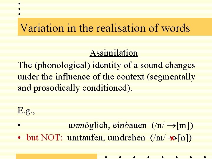
Variation in the realisation of words Assimilation The (phonological) identity of a sound changes under the influence of the context (segmentally and prosodically conditioned). E. g. , • unmöglich, einbauen (/n/ [m]) • but NOT: umtaufen, umdrehen (/m/ [n])

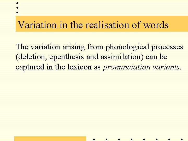
Variation in the realisation of words The variation arising from phonological processes (deletion, epenthesis and assimilation) can be captured in the lexicon as pronunciation variants.

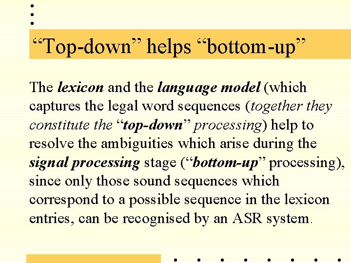
“Top-down” helps “bottom-up” The lexicon and the language model (which captures the legal word sequences (together they constitute the “top-down” processing) help to resolve the ambiguities which arise during the signal processing stage (“bottom-up” processing), since only those sound sequences which correspond to a possible sequence in the lexicon entries, can be recognised by an ASR system.

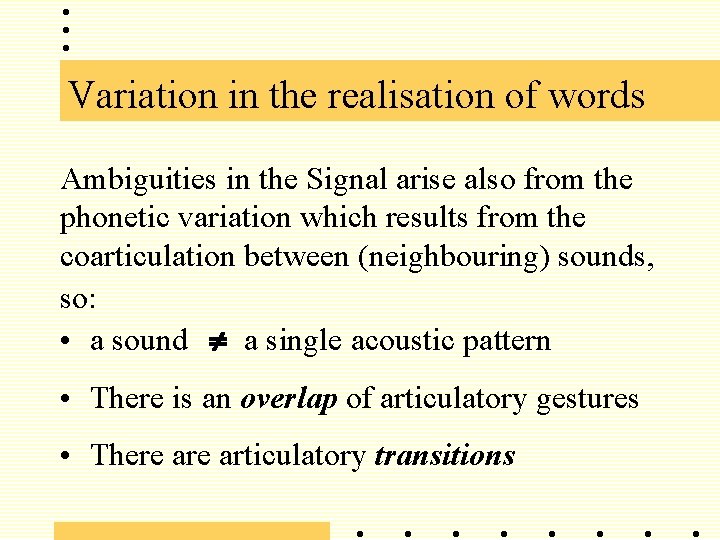
Variation in the realisation of words Ambiguities in the Signal arise also from the phonetic variation which results from the coarticulation between (neighbouring) sounds, so: • a sound a single acoustic pattern • There is an overlap of articulatory gestures • There articulatory transitions

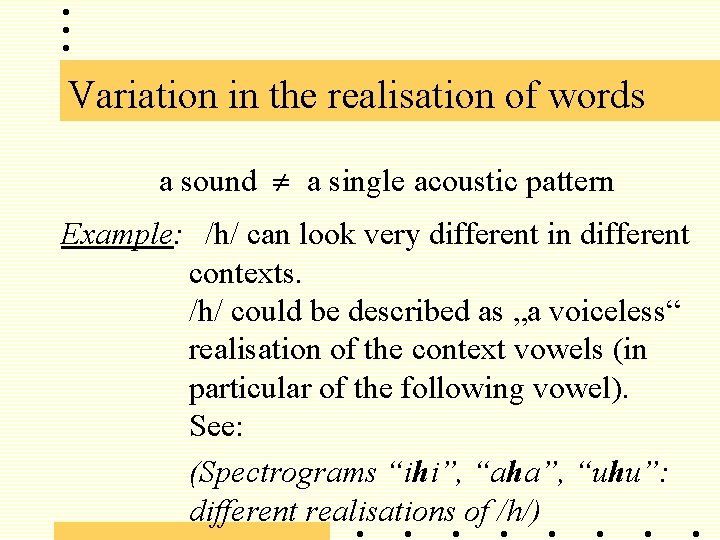
Variation in the realisation of words a sound a single acoustic pattern Example: /h/ can look very different in different contexts. /h/ could be described as „a voiceless“ realisation of the context vowels (in particular of the following vowel). See: (Spectrograms “ihi”, “aha”, “uhu”: different realisations of /h/)

Variation in the realisation of words [ i: h i: ] [ a: h a: ] [ u: hu: ]

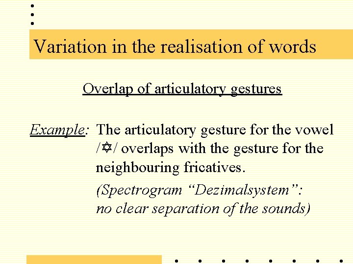
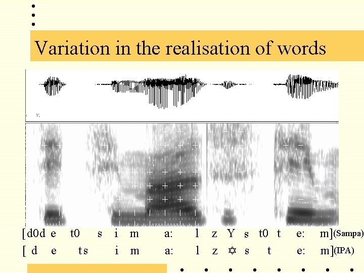
Variation in the realisation of words Overlap of articulatory gestures Example: The articulatory gesture for the vowel /Y/ overlaps with the gesture for the neighbouring fricatives. (Spectrogram “Dezimalsystem”: no clear separation of the sounds)

Variation in the realisation of words [ d 0 d e [ d e t 0 s ts i m a: a: l l z Y s t 0 t z Y s t e: e: m](Sampa) m](IPA)

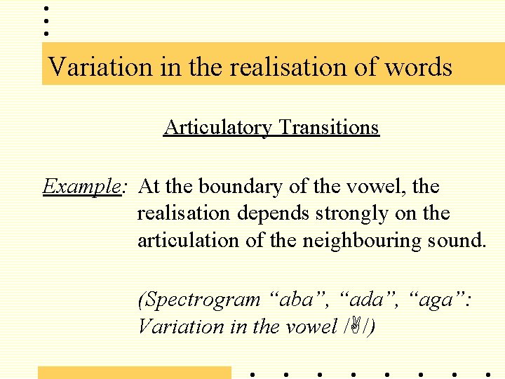
Variation in the realisation of words Articulatory Transitions Example: At the boundary of the vowel, the realisation depends strongly on the articulation of the neighbouring sound. (Spectrogram “aba”, “ada”, “aga”: Variation in the vowel /A/)

Variation in the realisation of words [ a: b 0 b a: ] [ a: d 0 d a: ] [ a: g 0 g a: ]

Variation in the realisation of words Human listeners don‘t normally have any problems with the variation in the Signal. For the Computer, it is a real challenge, because the variation in the realisation of a sound has to be captured in the acoustic models. To do that, statistical procedures are employed (mostly Hidden Markov Models).

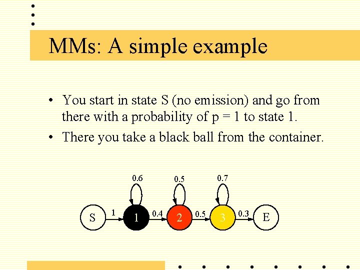
Markov-Modelling • Markov-Models consist of "states" which are connected by transitions. • When the Automat is in a particular state, it emits a symbol (e. g. an acoustic vector). stochastic • The transitions between the states are given Modelling probabilities. • Let‘s go through a simple example in which the states are containers with coloured balls.

MMs: A simple example • You start in state S (no emission) and go from there with a probability of p = 1 to state 1. • There you take a black ball from the container. 0. 6 S 1 1 0. 7 0. 5 0. 4 2 0. 5 3 0. 3 E

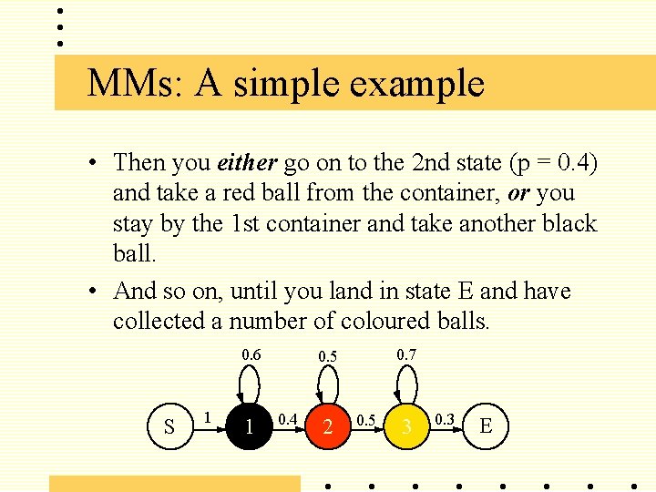
MMs: A simple example • Then you either go on to the 2 nd state (p = 0. 4) and take a red ball from the container, or you stay by the 1 st container and take another black ball. • And so on, until you land in state E and have collected a number of coloured balls. 0. 6 S 1 1 0. 7 0. 5 0. 4 2 0. 5 3 0. 3 E

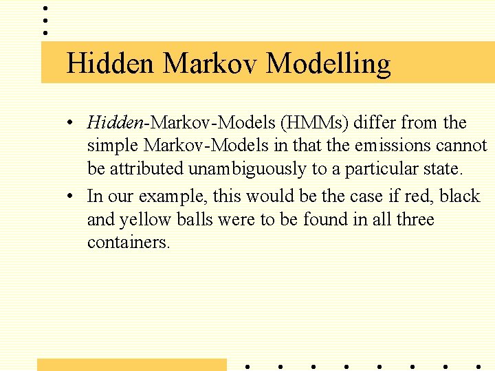
Hidden Markov Modelling • Hidden-Markov-Models (HMMs) differ from the simple Markov-Models in that the emissions cannot be attributed unambiguously to a particular state. • In our example, this would be the case if red, black and yellow balls were to be found in all three containers.

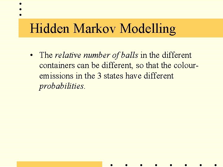
Hidden Markov Modelling • The relative number of balls in the different containers can be different, so that the colouremissions in the 3 states have different probabilities.

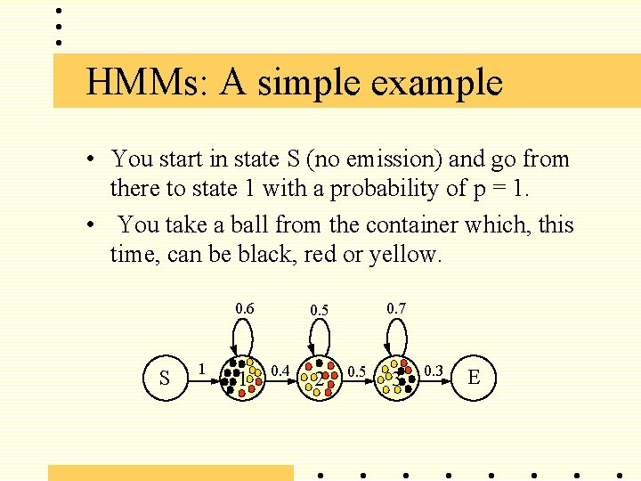
HMMs: A simple example • You start in state S (no emission) and go from there to state 1 with a probability of p = 1. • You take a ball from the container which, this time, can be black, red or yellow. 0. 6 S 1 1 0. 7 0. 5 0. 4 2 0. 5 3 0. 3 E

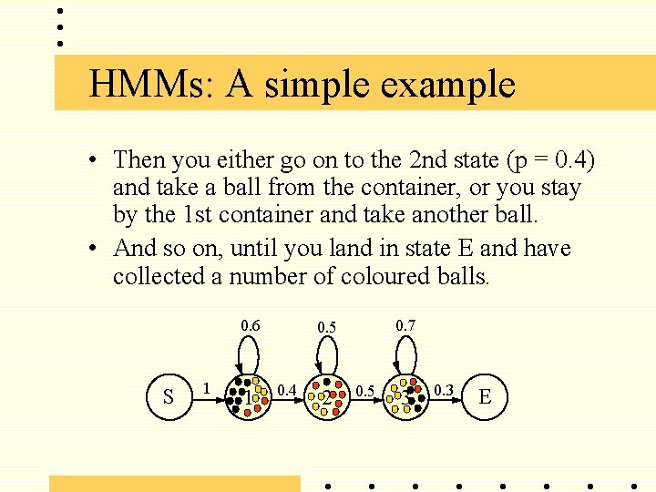
HMMs: A simple example • Then you either go on to the 2 nd state (p = 0. 4) and take a ball from the container, or you stay by the 1 st container and take another ball. • And so on, until you land in state E and have collected a number of coloured balls. 0. 6 S 1 1 0. 7 0. 5 0. 4 2 0. 5 3 0. 3 E

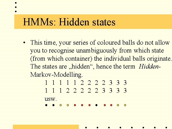
HMMs: Hidden states • This time, your series of coloured balls do not allow you to recognise unambiguously from which state (from which container) the individual balls originate. The states are „hidden“, hence the term Hidden. Markov-Modelling. 1 1 1 2 2 3 3 3 1 1 1 2 2 2 3 3 usw.

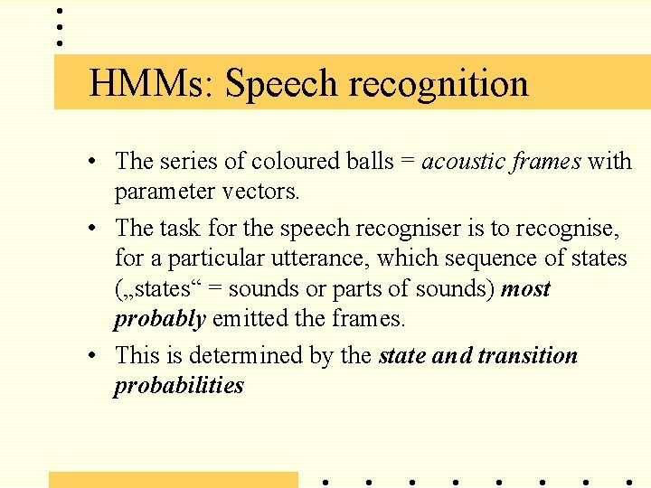
HMMs: Speech recognition • The series of coloured balls = acoustic frames with parameter vectors. • The task for the speech recogniser is to recognise, for a particular utterance, which sequence of states („states“ = sounds or parts of sounds) most probably emitted the frames. • This is determined by the state and transition probabilities

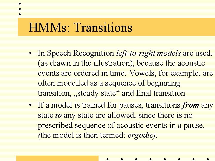
HMMs: Transitions • In Speech Recognition left-to-right models are used. (as drawn in the illustration), because the acoustic events are ordered in time. Vowels, for example, are often modelled as a sequence of beginning transition, „steady state“ and final transition. • If a model is trained for pauses, transitions from any state to any state are allowed, since there is no prescribed sequence of acoustic events in a pause. (the model is then termed: ergodic).

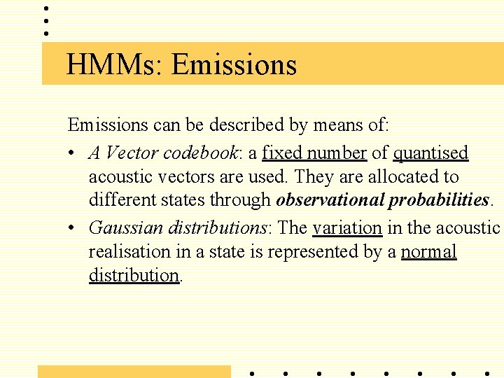
HMMs: Emissions can be described by means of: • A Vector codebook: a fixed number of quantised acoustic vectors are used. They are allocated to different states through observational probabilities. • Gaussian distributions: The variation in the acoustic realisation in a state is represented by a normal distribution.

HMMs: more complexe models More complex models can be used : • parallel states and „multiple mixtures“ can describe the variation in sound realisations better (speaker, dialect, context, etc. ). • Gaussian Mixtures: the systematic variation in the acoustic realisation of a state is represented by several normal distributions.

HMMs: Paucity of data? • Generalised triphones describe a sound in different contexts. The contexts are grouped (e. g. According to place of articulation or they are „data-driven“ by acoustic properties). • In this way, the demands on size of training corpus are reduced.

HMMs: Speech recognition • There can be several possible sequences of states arising from the same frame sequence. The sequences of states with the highest overall probability is sought (for this the Viterbi-Algorithm is used). • This is the same for all HMMs: The state sequence with the highest probability is recognised.

HMMs: Lexicon & Language model • HMMs are also used for continuous speech recognition. For that, one needs a lexicon and a language model as well as an acoustic model (Hidden-Markov-Model). • In the lexicon all the words (or morphemes) are listed which the system is expected to recognise. • In the language model the probabilities of all possible combinations of entries from Lexicon are specified.

HMMs: Lexicon • The entries in the lexicon consist of an orthographic word and its realisation as a sequence of HMMs for the sounds. • To deal better with variations in the pronunciation of words, pronunciation variants are sometimes included, taking reductions and deletions etc. Into consideration. • They reduce the distance between acoustic realisation and lexicon entry.

HMMs: Lexicon • However, the distance between the lexicon entries is also reduced, which can lead to greater confusion between entries. For that reason it is usually only the most frequent variants that are included, e. g. Function words.

HMMs: Language model • The language model can be implemented either as a system of rules (like a linguistic grammar) or as a probabilistic system. • Rule systems have the advantage that they lead to a better understanding of the linguistic properties of utterances (just as knowledge based sound recognition can lead to a better understanding of the phonetic properties of sounds)

HMMs: Language model • Probabilistic systems model realised utterances (rather than projected utterances). They calculate probabilities of the transitions between lexicon entries. They are less generalising, but need very large amounts of data as training material. Assuming that the Test conditions agree with the training conditions (type of text , lexical domain, recording conditions, etc. ) they describe the observed speaker behaviour extremely well.

Literature: • Van Alphen, P. und D. van Bergem (1989). „Markov models and their application in speech recognition, “ Proceedings Institute of Phonetic Sciences, University of Amsterdam 13, 1 -26. • Holmes, J. (1988). Speech Synthesis and Recognition (Kap. 8). Wokingham (Berks. ): Van Nostrand Reinhold, 129 -152. • Holmes, J. (1991). Spracherkennung und Sprachsynthese (Kap. 8). München: Oldenburg.

Literature: • Cox, S. (1988). „Hidden Markov models for automatic speech recognition: theory and application, “ Br. Telecom techn. Journal 6(2), 105115. • Lee, K. -F. (1989). „Hidden Markov modelling: past, present, future, “ Proc. Eurospeech 1989, vol. 1, 148 -155.