Search and Decoding in Speech Recognition Automatic Speech
- Slides: 37

Search and Decoding in Speech Recognition Automatic Speech Recognition Advanced Topics

Speech Recognition Systems Architecture u The task of speech recognition is to take as input an acoustic waveform and produce as output a string of words. u HMM-based speech recognition systems view this task using the metaphor of the noisy channel. The intuition of the noisy channel model is to treat the acoustic waveform as a “noisy” version of the string of words, i. e. . a version that has been passed through a noisy communications channel 11/3/2020 Veton Këpuska 2

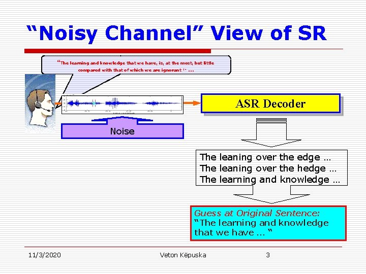
“Noisy Channel” View of SR “The learning and knowledge that we have, is, at the most, but little compared with that of which we are ignorant !” … ASR Decoder Noise The leaning over the edge … The leaning over the hedge … The learning and knowledge … Guess at Original Sentence: “The learning and knowledge that we have … “ 11/3/2020 Veton Këpuska 3

“Noisy Channel” View of SR u This channel introduces “noise” which makes it hard to recognize the “true” string of words. Our goal is then to build a model of the channel so that we can figure out how it modified this “true” sentence and hence recover it. u “Noise Channel” view absorbs all variability's of the speech mentioned earlier including true noise. u Having insight of the noisy channel model means that we know how the channel distorts the source, we could find the correct source sentence for a waveform by taking every possible sentence in the language, running each sentence through our noisy channel model, and seeing if it matches the output. u We then select the best matching source sentence as our desired source sentence. 11/3/2020 Veton Këpuska 4

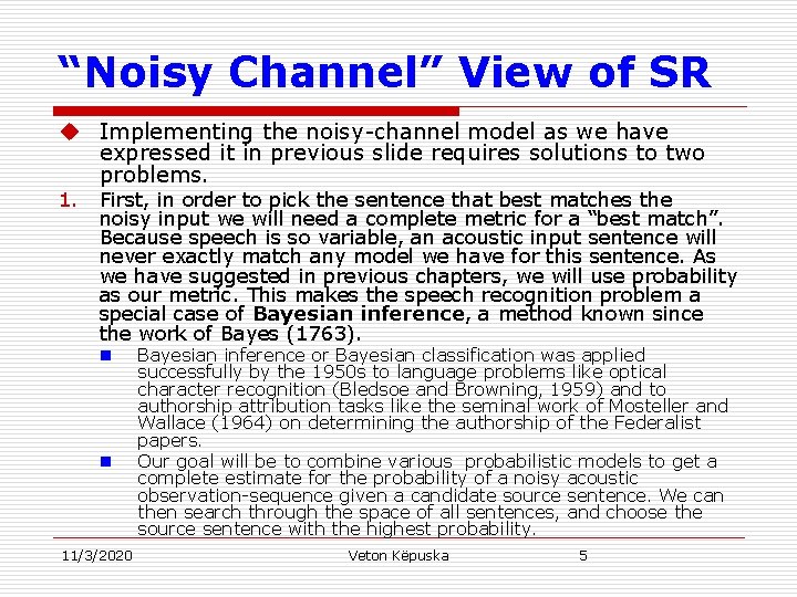
“Noisy Channel” View of SR u Implementing the noisy-channel model as we have expressed it in previous slide requires solutions to two problems. 1. First, in order to pick the sentence that best matches the noisy input we will need a complete metric for a “best match”. Because speech is so variable, an acoustic input sentence will never exactly match any model we have for this sentence. As we have suggested in previous chapters, we will use probability as our metric. This makes the speech recognition problem a special case of Bayesian inference, a method known since the work of Bayes (1763). n n 11/3/2020 Bayesian inference or Bayesian classification was applied successfully by the 1950 s to language problems like optical character recognition (Bledsoe and Browning, 1959) and to authorship attribution tasks like the seminal work of Mosteller and Wallace (1964) on determining the authorship of the Federalist papers. Our goal will be to combine various probabilistic models to get a complete estimate for the probability of a noisy acoustic observation-sequence given a candidate source sentence. We can then search through the space of all sentences, and choose the source sentence with the highest probability. Veton Këpuska 5

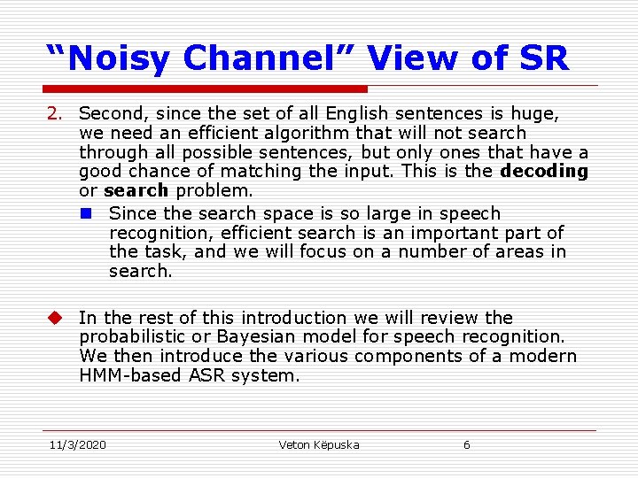
“Noisy Channel” View of SR 2. Second, since the set of all English sentences is huge, we need an efficient algorithm that will not search through all possible sentences, but only ones that have a good chance of matching the input. This is the decoding or search problem. n Since the search space is so large in speech recognition, efficient search is an important part of the task, and we will focus on a number of areas in search. u In the rest of this introduction we will review the probabilistic or Bayesian model for speech recognition. We then introduce the various components of a modern HMM-based ASR system. 11/3/2020 Veton Këpuska 6

Speech Recognition Information Theoretic Approach to ASR

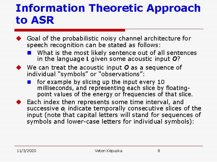
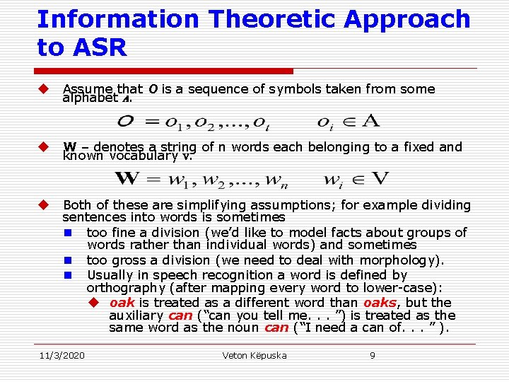
Information Theoretic Approach to ASR u Goal of the probabilistic noisy channel architecture for speech recognition can be stated as follows: n What is the most likely sentence out of all sentences in the language L given some acoustic input O? u We can treat the acoustic input O as a sequence of individual “symbols” or “observations”: n for example by slicing up the input every 10 milliseconds, and representing each slice by floatingpoint values of the energy or frequencies of that slice. u Each index then represents some time interval, and successive oi indicate temporally consecutive slices of the input (note that capital letters will stand for sequences of symbols and lower-case letters for individual symbols): 11/3/2020 Veton Këpuska 8

Information Theoretic Approach to ASR u Assume that O is a sequence of symbols taken from some alphabet A. u W – denotes a string of n words each belonging to a fixed and known vocabulary V. u Both of these are simplifying assumptions; for example dividing sentences into words is sometimes n too fine a division (we’d like to model facts about groups of words rather than individual words) and sometimes n too gross a division (we need to deal with morphology). n Usually in speech recognition a word is defined by orthography (after mapping every word to lower-case): u oak is treated as a different word than oaks, but the auxiliary can (“can you tell me. . . ”) is treated as the same word as the noun can (“I need a can of. . . ” ). 11/3/2020 Veton Këpuska 9

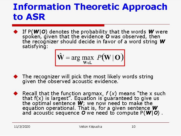
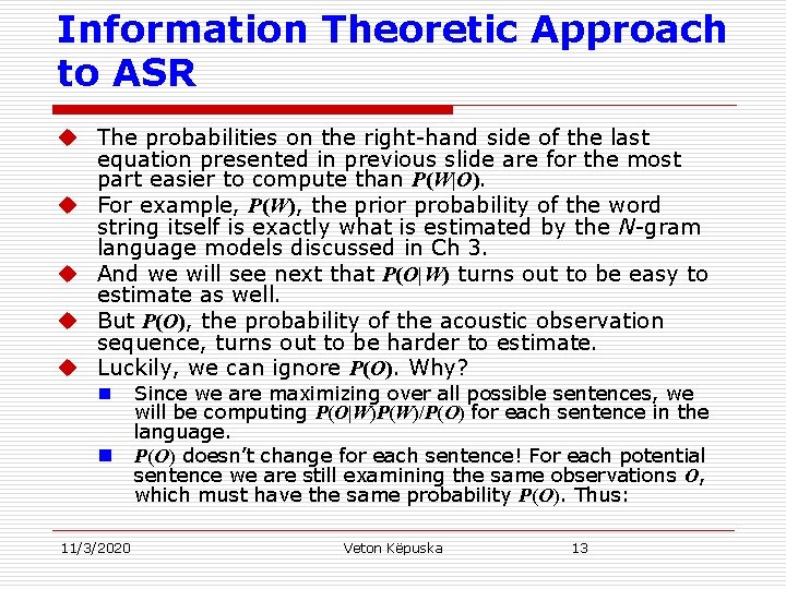
Information Theoretic Approach to ASR u If P(W|O) denotes the probability that the words W were spoken, given that the evidence O was observed, then the recognizer should decide in favor of a word string W satisfying: u The recognizer will pick the most likely words string given the observed acoustic evidence. u Recall that the function argmaxx f (x) means “the x such that f(x) is largest”. Equation is guaranteed to give us the optimal sentence W; we now need to make the equation operational. That is, for a given sentence W and acoustic sequence O we need to compute P(W|O). 11/3/2020 Veton Këpuska 10

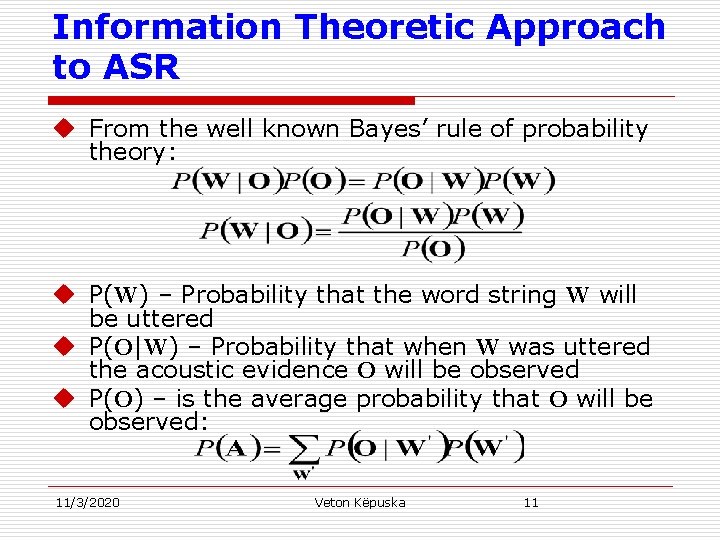
Information Theoretic Approach to ASR u From the well known Bayes’ rule of probability theory: u P(W) – Probability that the word string W will be uttered u P(O|W) – Probability that when W was uttered the acoustic evidence O will be observed u P(O) – is the average probability that O will be observed: 11/3/2020 Veton Këpuska 11

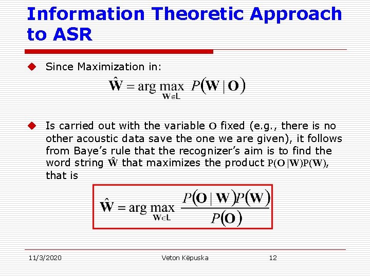
Information Theoretic Approach to ASR u Since Maximization in: u Is carried out with the variable O fixed (e. g. , there is no other acoustic data save the one we are given), it follows from Baye’s rule that the recognizer’s aim is to find the word string Ŵ that maximizes the product P(O |W)P(W), that is 11/3/2020 Veton Këpuska 12

Information Theoretic Approach to ASR u The probabilities on the right-hand side of the last equation presented in previous slide are for the most part easier to compute than P(W|O). u For example, P(W), the prior probability of the word string itself is exactly what is estimated by the N-gram language models discussed in Ch 3. u And we will see next that P(O|W) turns out to be easy to estimate as well. u But P(O), the probability of the acoustic observation sequence, turns out to be harder to estimate. u Luckily, we can ignore P(O). Why? n n 11/3/2020 Since we are maximizing over all possible sentences, we will be computing P(O|W)P(W)/P(O) for each sentence in the language. P(O) doesn’t change for each sentence! For each potential sentence we are still examining the same observations O, which must have the same probability P(O). Thus: Veton Këpuska 13

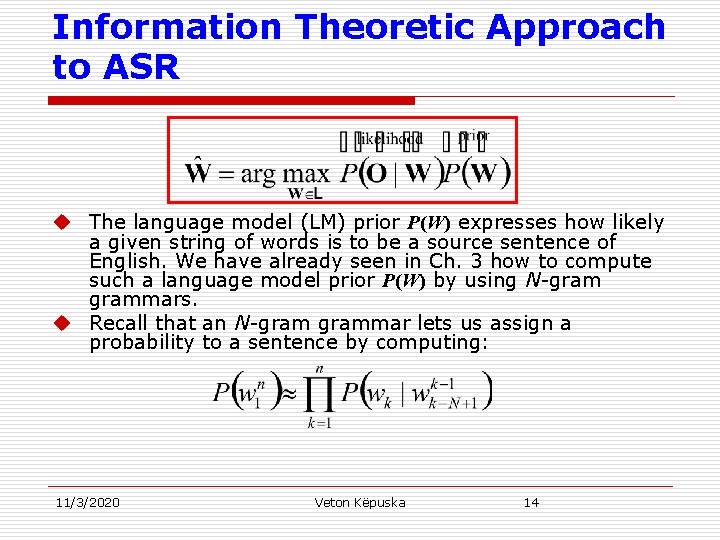
Information Theoretic Approach to ASR u The language model (LM) prior P(W) expresses how likely a given string of words is to be a source sentence of English. We have already seen in Ch. 3 how to compute such a language model prior P(W) by using N-grammars. u Recall that an N-grammar lets us assign a probability to a sentence by computing: 11/3/2020 Veton Këpuska 14

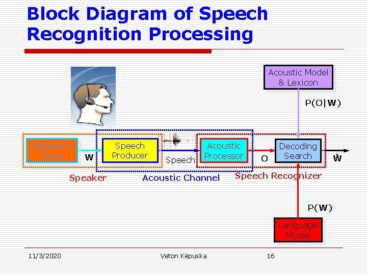
Information Theoretic Approach to ASR u This chapter will show the HMM can be used to build an Acoustic Model (AM) which computes the likelihood P(O|W). u Given the AM and LM probabilities, the probabilistic model can be operationalized in a search algorithm so as to compute the maximum probability word string for a given acoustic waveform. u Figure presented in the next slide shows a rough block diagram of how the computation of the prior and likelihood fits into a recognizer decoding a sentence. 11/3/2020 Veton Këpuska 15

Block Diagram of Speech Recognition Processing Acoustic Model & Lexicon P(O|W) Speaker's Mind W Speaker Speech Producer Speech Acoustic Processor Acoustic Channel O Decoding Search Speech Recognizer P(W) Language Model 11/3/2020 Veton Këpuska 16 Ŵ

Hierarchical Algorithm u It is not possible to apply very expensive algorithms in the speech recognition process, such as 4 -gram, 5 -gram, or even parser-based language models, or context-dependent phone models that can see two or three phones into the future or past. n n 11/3/2020 There a huge number of potential transcriptions sentences for any given waveform, and it’s too expensive (in time, space, or both) to apply these powerful algorithms to every single candidate. Instead, we’ll introduce multipass decoding algorithms in which efficient but dumber decoding algorithms produce shortlists of potential candidates to be rescored by slow but smarter algorithms. We’ll also introduce the context-dependent acoustic model, which is one of these smarter knowledge sources that turns out to be essential in large vocabulary speech recognition. We’ll also briefly introduce the important topics of discriminative training and the modeling of variation. Veton Këpuska 17

Multipass Decoding: N-Best Lists and Lattices u The previous chapters we applied the Viterbi algorithm for HMM decoding. u There are two main limitations of the Viterbi decoder. 1. The Viterbi decoder does not actually compute the sequence of words which is most probable given the input acoustics. Instead, it computes an approximation to this: the sequence of states (i. e. , phones or subphones) which is most probable given the input. 2. A second problem with the Viterbi decoder is that it is impossible or expensive for it to take advantage of many useful knowledge sources. 11/3/2020 Veton Këpuska 18

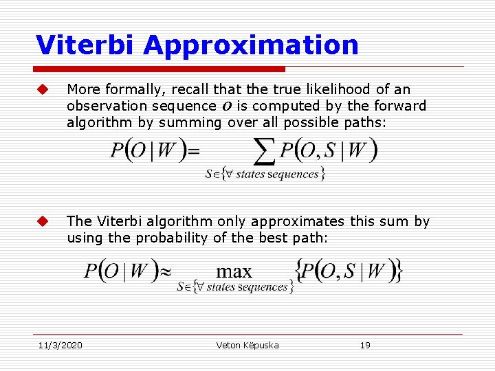
Viterbi Approximation u More formally, recall that the true likelihood of an observation sequence O is computed by the forward algorithm by summing over all possible paths: u The Viterbi algorithm only approximates this sum by using the probability of the best path: 11/3/2020 Veton Këpuska 19

Viterbi Approximation u It turns out that this Viterbi approximation is not too bad, since the most probable sequence of phones usually turns out to correspond to the most probable sequence of words. But not always. u Consider a speech recognition system whose lexicon has multiple pronunciations for each word. Suppose the correct word sequence includes a word with very many pronunciations. Since the probabilities leaving the start arc of each word must sum to 1. 0, each of these pronunciationpaths through this multiple pronunciation HMM word model will have a smaller probability than the path through a word with only a single pronunciation path. Thus because the Viterbi decoder can only follow one of these pronunciation paths, it may ignore this many-pronunciation word in favor of an incorrect word with only one pronunciation path. u In essence, the Viterbi approximation penalizes words with many pronunciations. 11/3/2020 Veton Këpuska 20

Incorporation of Useful Knowledge Sources Problem u For example the Viterbi algorithm as we have defined it cannot take complete advantage of any language model more complex than a bigrammar. u This is because of the fact that a trigrammar, for example, violates the dynamic programming invariant. Recall that this invariant is the simplifying (but incorrect) assumption that if the ultimate best path for the entire observation sequence happens to go through a state qi, that this best path must include the best path up to and including state qj. u Since a trigrammar allows the probability of a word to be based on the two previous words, it is possible that the best trigram-probability path for the sentence may go through a word but not include the best path to that word. Such a situation could occur if a particular word wx has a high trigram probability given wy, wz, but that conversely the best path to wy didn’t include wz (i. e. , P(wy|wq, wz) was low for all q). 11/3/2020 Veton Këpuska 21

Solutions 1. Multiple-pass Decoding: u 2. The most common solution is to modify the Viterbi decoder to return multiple potential utterances, instead of just the single best, and then use other high-level language model or pronunciation modeling algorithms to re-rank these multiple outputs (Schwartz and Austin, 1991; Soong and Huang, 1990; Murveit et al. , 1993). Stack Decoder: u 11/3/2020 The second solution is to employ a completely different decoding algorithm, such as the stack decoder, or A∗ decoder (Jelinek, 1969; Jelinek et al. , 1975). Veton Këpuska 22

Multipass Decoding: N-Best Lists and Lattices

Multiple-pass Decoding u In multiple-pass decoding we break up the decoding process into two stages. n In the first stage we use fast, efficient knowledge sources or algorithms to perform a non-optimal search. u So for example we might use an unsophisticated but time-and-space efficient language model like a bigram, or use simplified acoustic models. n In the second decoding pass we can apply more sophisticated but slower decoding algorithms on a reduced search space. n The interface between these passes is an N-best list or word lattice. 11/3/2020 Veton Këpuska 24

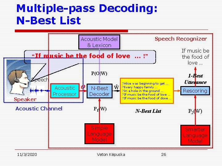
Multiple-pass Decoding: N-Best List u The simplest algorithm for multipass decoding is to modify the Viterbi algorithm to return the N-best sentences (word sequences) for a given speech input. n n 11/3/2020 Suppose for example a bigrammar is used with such an N -best-Viterbi algorithm to return the 1000 most highlyprobable sentences, each with their Acoustic Model (AM) likelihood and Language Model (LM) prior score. This 1000 -best list can now be passed to a more sophisticated language model like a trigrammar. This new LM is used to replace the bigram LM score of each hypothesized sentence with a new trigram LM probability. These priors can be combined with the acoustic likelihood of each sentence to generate a new posterior probability for each sentence. Sentences are thus rescored and re-ranked using this more sophisticated probability. Fig. in the next slide depicts the idea behind this algorithm. Veton Këpuska 25

Multiple-pass Decoding: N-Best List Speech Recognizer Acoustic Model & Lexicon If music be the food of love … “If music be the food of love … !” P(O|W) Speech Speaker Acoustic Processor Acoustic Channel O N-Best Ŵ Decoder ? Alice was beginning to get … ? Every happy family … ? In a hole in the ground … ? If music be the food of love … ? If music be the food of dove … P 1(W) N-Best List Veton Këpuska Rescoring P 2(W) Simple Language Model 11/3/2020 1 -Best Utterance Smarter Language Model 26

Multiple-pass Decoding: N-Best List u u There a number of algorithms for augmenting the Viterbi algorithm to generate N-best hypotheses. It turns out that there is no polynomial-time admissible algorithm for finding the N most likely hypotheses (Young, 1984). There are however, a number of approximate (non-admissible) algorithms; we will introduce just one of them, the “Exact N-best” algorithm of Schwartz and Chow (1990). In Exact N-best, instead of each state maintaining a single path/backtrace, we maintain up to N different paths for each state. But we’d like to insure that these paths correspond to different word paths; we don’t want to waste our N paths on different state sequences that map to the same words. To do this, we keep for each path the word history, the entire sequence of words up to the current word/state. If two paths with the same word history come to a state at the same time, we merge the paths and sum the path probabilities. To keep the N best word sequences, the resulting algorithm requires O(N) times the normal Viterbi time. We’ll see this merging of paths again when we introducing decoding for statistical machine translation, where it is called hypothesis recombination. 11/3/2020 Veton Këpuska 27

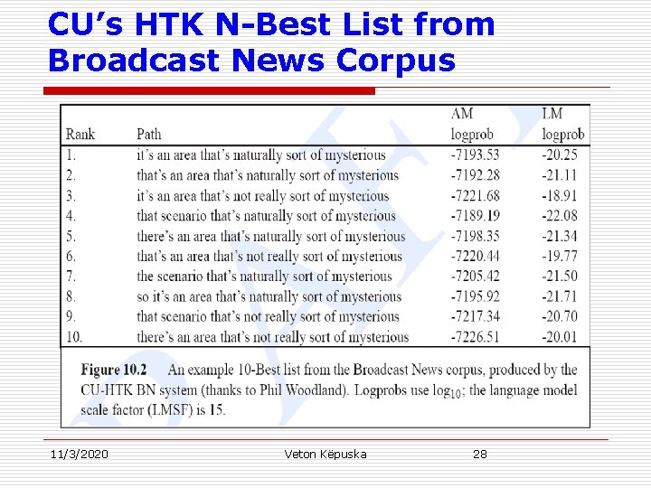
CU’s HTK N-Best List from Broadcast News Corpus 11/3/2020 Veton Këpuska 28

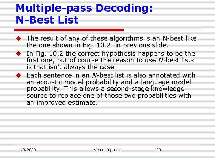
Multiple-pass Decoding: N-Best List u The result of any of these algorithms is an N-best like the one shown in Fig. 10. 2. in previous slide. u In Fig. 10. 2 the correct hypothesis happens to be the first one, but of course the reason to use N-best lists is that isn’t always the case. u Each sentence in an N-best list is also annotated with an acoustic model probability and a language model probability. This allows a second-stage knowledge source to replace one of those two probabilities with an improved estimate. 11/3/2020 Veton Këpuska 29

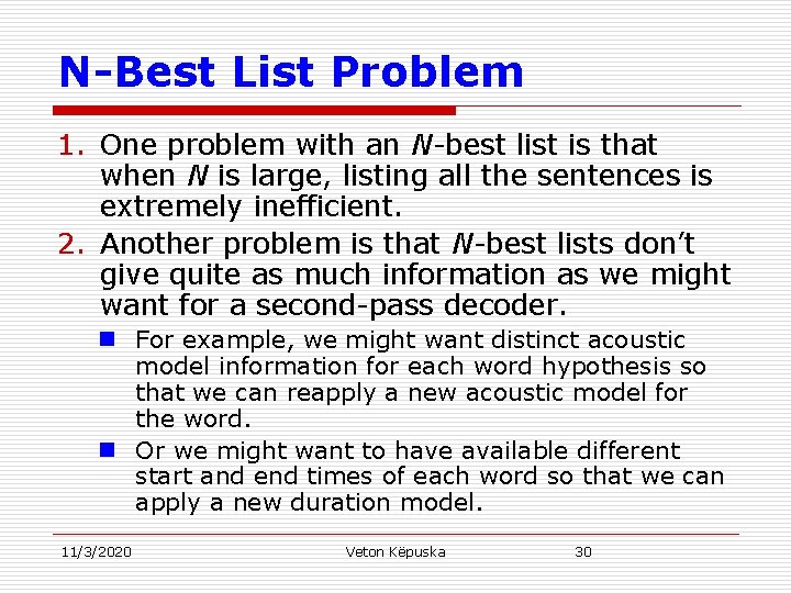
N-Best List Problem 1. One problem with an N-best list is that when N is large, listing all the sentences is extremely inefficient. 2. Another problem is that N-best lists don’t give quite as much information as we might want for a second-pass decoder. n For example, we might want distinct acoustic model information for each word hypothesis so that we can reapply a new acoustic model for the word. n Or we might want to have available different start and end times of each word so that we can apply a new duration model. 11/3/2020 Veton Këpuska 30

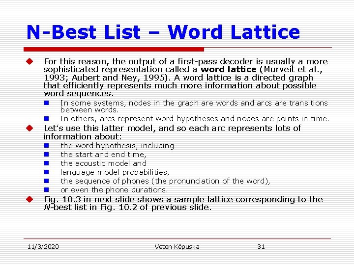
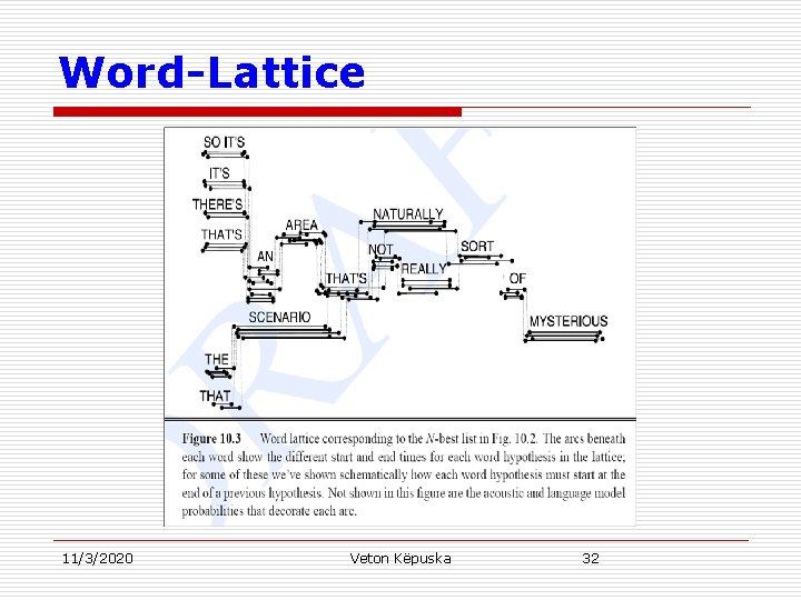
N-Best List – Word Lattice u For this reason, the output of a first-pass decoder is usually a more sophisticated representation called a word lattice (Murveit et al. , 1993; Aubert and Ney, 1995). A word lattice is a directed graph that efficiently represents much more information about possible word sequences. n In some systems, nodes in the graph are words and arcs are transitions between words. In others, arcs represent word hypotheses and nodes are points in time. n n n the word hypothesis, including the start and end time, the acoustic model and language model probabilities, the sequence of phones (the pronunciation of the word), or even the phone durations. n u u Let’s use this latter model, and so each arc represents lots of information about: Fig. 10. 3 in next slide shows a sample lattice corresponding to the N-best list in Fig. 10. 2 of previous slide. 11/3/2020 Veton Këpuska 31

Word-Lattice 11/3/2020 Veton Këpuska 32

Word-Lattice u u u The fact that each word hypothesis in a lattice is augmented separately with its acoustic model likelihood and language model probability allows us to rescore any path through the lattice, using n n either a more sophisticated language model or a more sophisticated acoustic model. n The lattice error rate is the word error rate we get if we chose the lattice path (the sentence) that has the lowest word error rate. Because it relies on perfect knowledge of which path to pick, we call this an oracle error rate, since we need some oracle to tell us which sentence/path to pick. As with N-best lists, the goal of this rescoring is to replace the 1 best utterance with a different utterance that perhaps had a lower score on the first decoding pass. For this second-pass knowledge source to get perfect word error rate, the actual correct sentence would have to be in the lattice or N-best list. If the correct sentence isn’t there, the rescoring knowledge source can’t find it. Thus it is important when working with a lattice or N-best list to consider the baseline lattice error rate (Woodland et al. , 1995; Ortmanns et al. , 1997): the lower bound word error rate from the lattice. 11/3/2020 Veton Këpuska 33

Lattice Density u Another important lattice concept is the lattice density, which is the number of edges in a lattice divided by the number of words in the reference transcript. n As we saw schematically in Fig. 10. 3, real lattices are often extremely dense, with many copies of individual word hypotheses at slightly different start and end times. n Because of this density, lattices are often pruned. 11/3/2020 Veton Këpuska 34

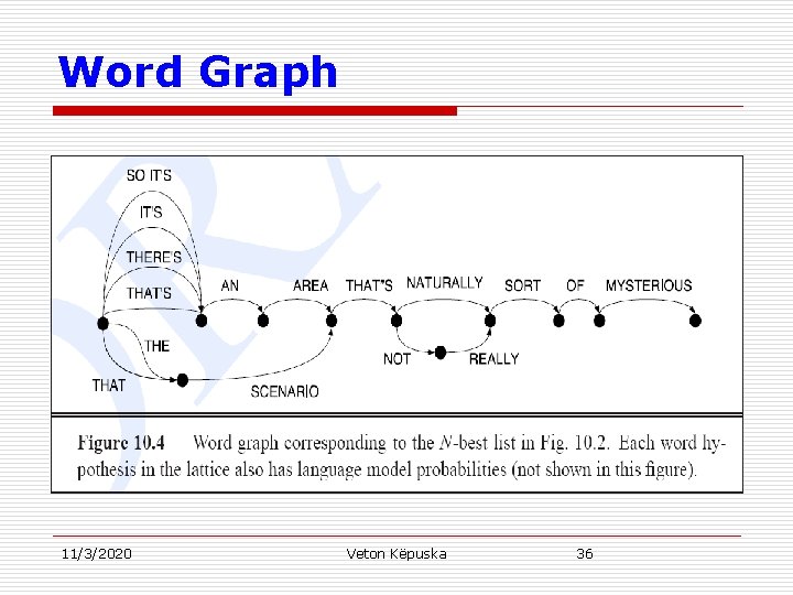
Word Graph u u u Besides pruning, lattices are often simplified into a different, more schematic kind of lattice that is sometimes called a word graph or finite state machine, although often it’s still just referred to as a word lattice. In these word graphs, the timing information is removed and multiple overlapping copies of the same word are merged. The timing of the words is left implicit in the structure of the graph. In addition, the acoustic model likelihood information is removed, leaving only the language model probabilities. The resulting graph is a weighted Finite State Automaton (FSA), which is a natural extension of an N-gram language model; the word graph corresponding to Fig. 10. 3 is shown in Fig. 10. 4 in the next slide. This word graph can in fact be used as the language model for another decoding pass. Since such a wordgraph language model vastly restricts the search space, it can make it possible to use a complicated acoustic model which is too slow to use in first-pass decoding. 11/3/2020 Veton Këpuska 35

Word Graph 11/3/2020 Veton Këpuska 36

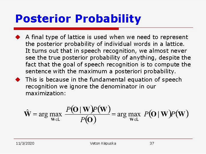
Posterior Probability u A final type of lattice is used when we need to represent the posterior probability of individual words in a lattice. It turns out that in speech recognition, we almost never see the true posterior probability of anything, despite the fact that the goal of speech recognition is to compute the sentence with the maximum a posteriori probability. u This is because in the fundamental equation of speech recognition we ignore the denominator in our maximization: 11/3/2020 Veton Këpuska 37