afex Analysis of Factorial Experiments in R Henrik

afex – Analysis of Factorial Experiments in R Henrik Singmann Universität Zürich

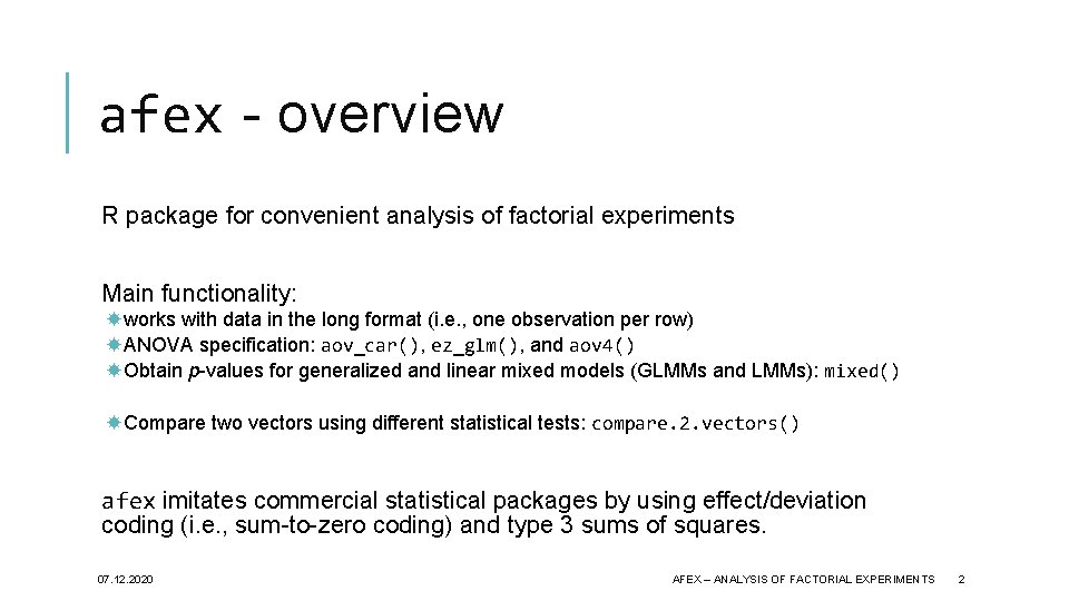
afex - overview R package for convenient analysis of factorial experiments Main functionality: works with data in the long format (i. e. , one observation per row) ANOVA specification: aov_car(), ez_glm(), and aov 4() Obtain p-values for generalized and linear mixed models (GLMMs and LMMs): mixed() Compare two vectors using different statistical tests: compare. 2. vectors() afex imitates commercial statistical packages by using effect/deviation coding (i. e. , sum-to-zero coding) and type 3 sums of squares. 07. 12. 2020 AFEX – ANALYSIS OF FACTORIAL EXPERIMENTS 2

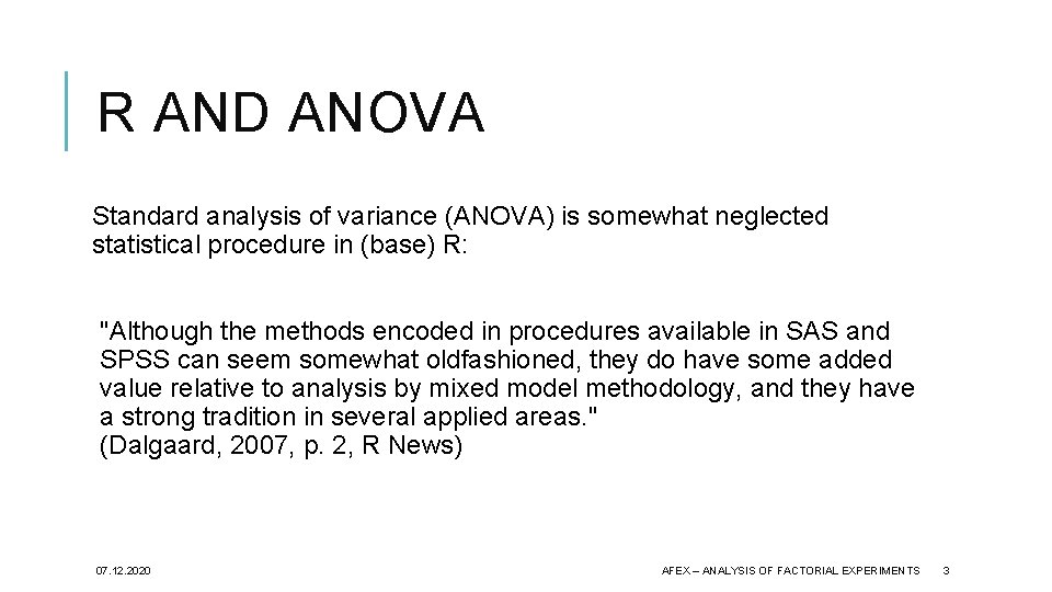
R AND ANOVA Standard analysis of variance (ANOVA) is somewhat neglected statistical procedure in (base) R: "Although the methods encoded in procedures available in SAS and SPSS can seem somewhat oldfashioned, they do have some added value relative to analysis by mixed model methodology, and they have a strong tradition in several applied areas. " (Dalgaard, 2007, p. 2, R News) 07. 12. 2020 AFEX – ANALYSIS OF FACTORIAL EXPERIMENTS 3

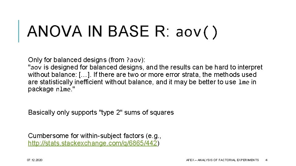
ANOVA IN BASE R: aov() Only for balanced designs (from ? aov): "aov is designed for balanced designs, and the results can be hard to interpret without balance: […]. If there are two or more error strata, the methods used are statistically inefficient without balance, and it may be better to use lme in package nlme. " Basically only supports "type 2" sums of squares Cumbersome for within-subject factors (e. g. , http: //stats. stackexchange. com/q/6865/442) 07. 12. 2020 AFEX – ANALYSIS OF FACTORIAL EXPERIMENTS 4

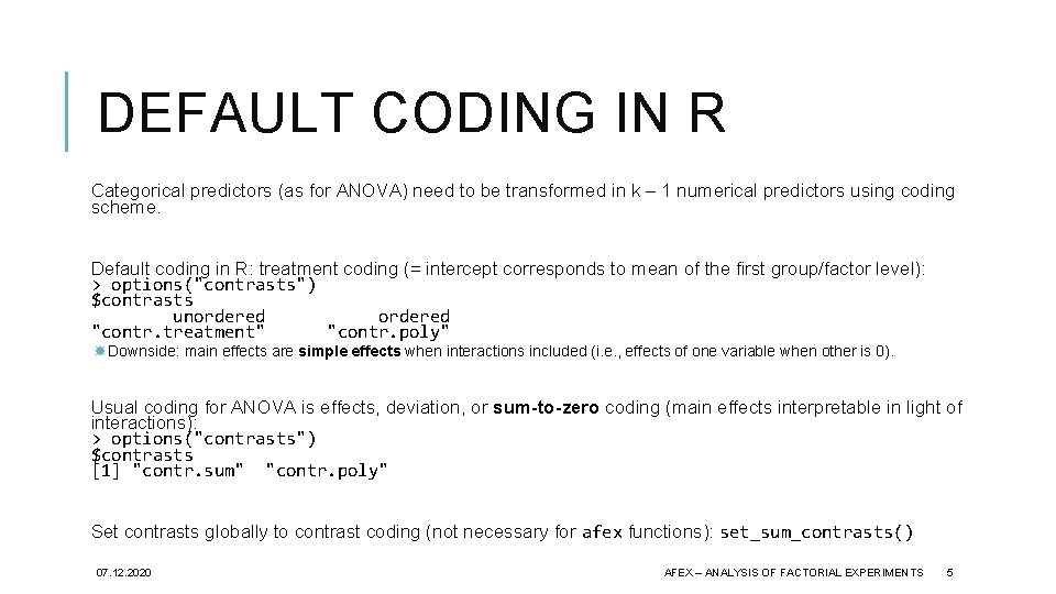
DEFAULT CODING IN R Categorical predictors (as for ANOVA) need to be transformed in k – 1 numerical predictors using coding scheme. Default coding in R: treatment coding (= intercept corresponds to mean of the first group/factor level): > options("contrasts") $contrasts unordered "contr. treatment" "contr. poly" Downside: main effects are simple effects when interactions included (i. e. , effects of one variable when other is 0). Usual coding for ANOVA is effects, deviation, or sum-to-zero coding (main effects interpretable in light of interactions): > options("contrasts") $contrasts [1] "contr. sum" "contr. poly" Set contrasts globally to contrast coding (not necessary for afex functions): set_sum_contrasts() 07. 12. 2020 AFEX – ANALYSIS OF FACTORIAL EXPERIMENTS 5

ALTERNATIVES TO AOV() car: : Anova() from John Fox can handle any number of between- and within-subjects factors allows for so called "type 2" and "type 3" sums of squares. but, relatively uncomfortable for within-subject factors, as data needs to be in wide format (i. e. , one participant per row) ez (by Mike Lawrence) provides a wrapper for car: : Anova(), ez. ANOVA(), but does not replicate commercial packages without fine-tuning afex is another car wrapper: aov_car() provides an aov() like formula interface aov_ez() specification of factors using character vectors aov_4() specification using lme 4: : lmer type syntax. afex automatically sets default contrasts to contr. sum (i. e. , sum-to-zero or deviation coding) 07. 12. 2020 AFEX – ANALYSIS OF FACTORIAL EXPERIMENTS 6

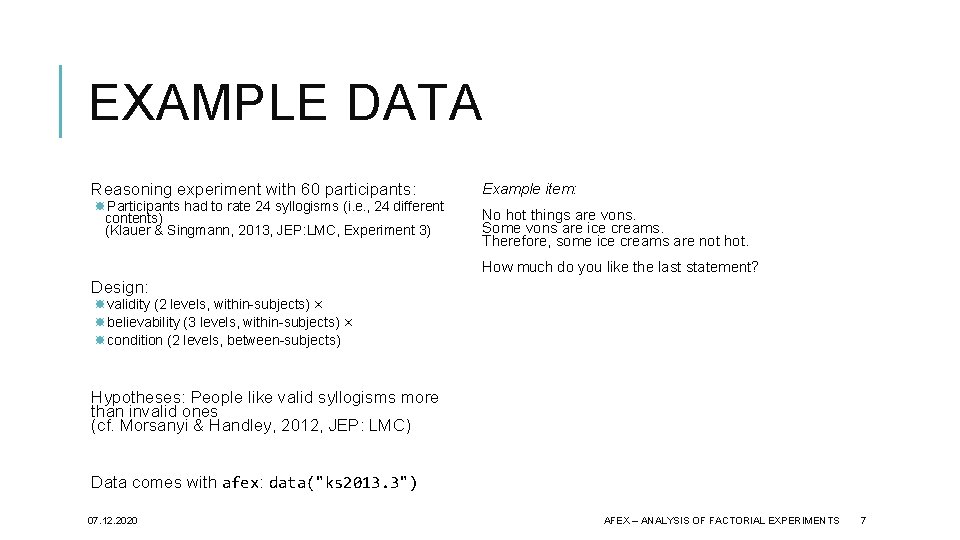
EXAMPLE DATA Reasoning experiment with 60 participants: Participants had to rate 24 syllogisms (i. e. , 24 different contents) (Klauer & Singmann, 2013, JEP: LMC, Experiment 3) Example item: No hot things are vons. Some vons are ice creams. Therefore, some ice creams are not hot. How much do you like the last statement? Design: validity (2 levels, within-subjects) × believability (3 levels, within-subjects) × condition (2 levels, between-subjects) Hypotheses: People like valid syllogisms more than invalid ones (cf. Morsanyi & Handley, 2012, JEP: LMC) Data comes with afex: data("ks 2013. 3") 07. 12. 2020 AFEX – ANALYSIS OF FACTORIAL EXPERIMENTS 7

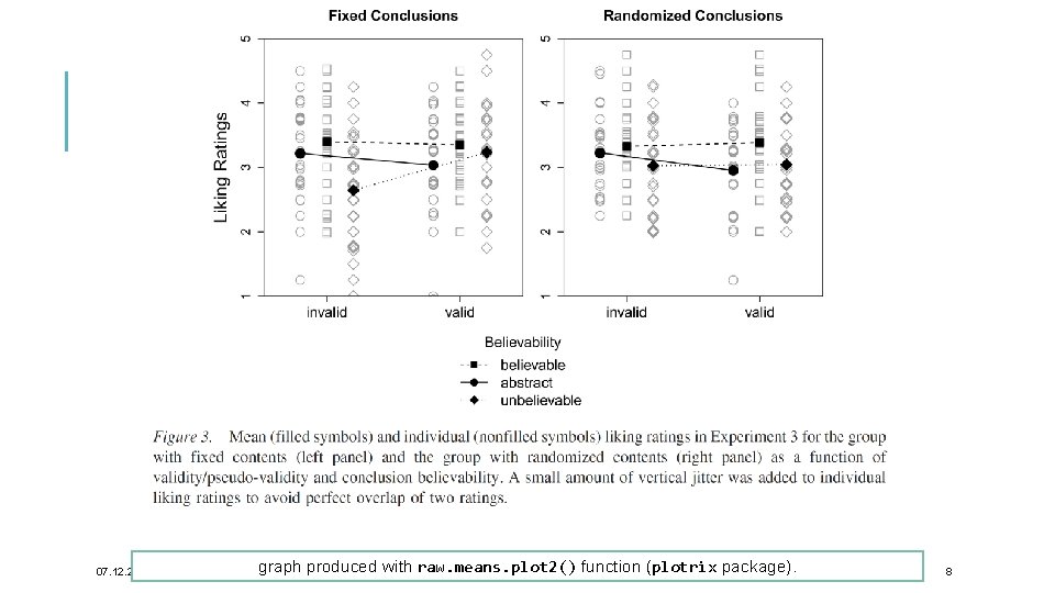
07. 12. 2020 graph produced with raw. means. plot 2() function (plotrix package). AN INTRODUCTION TO R 8

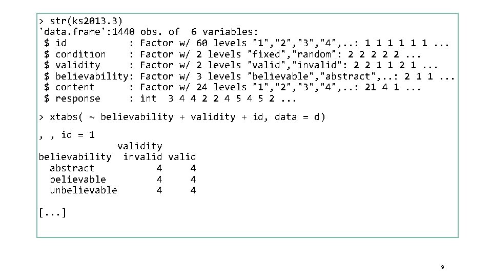
> str(ks 2013. 3) 'data. frame': 1440 $ id : $ condition : $ validity : $ believability: $ content : $ response : obs. of 6 variables: Factor w/ 60 levels "1", "2", "3", "4", . . : 1 1 1. . . Factor w/ 2 levels "fixed", "random": 2 2 2. . . Factor w/ 2 levels "valid", "invalid": 2 2 1 1 2 1. . . Factor w/ 3 levels "believable", "abstract", . . : 2 1 1. . . Factor w/ 24 levels "1", "2", "3", "4", . . : 21 4 1. . . int 3 4 4 2 2 4 5 2. . . > xtabs( ~ believability + validity + id, data = d) , , id = 1 validity believability invalid abstract 4 4 believable 4 4 unbelievable 4 4 [. . . ] 9

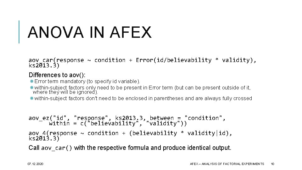
ANOVA IN AFEX aov_car(response ~ condition + Error(id/believability * validity), ks 2013. 3) Differences to aov(): Error term mandatory (to specify id variable). within-subject factors only need to be present in Error term (but can be present outside of it, where they will be ignored). within-subject factors don't need to be enclosed in parentheses and are always fully crossed aov_ez("id", "response", ks 2013. 3, between = "condition", within = c("believability", "validity")) aov_4(response ~ condition + (believability * validity|id), ks 2013. 3) Call aov_car() with the respective formula and produce identical output. 07. 12. 2020 AFEX – ANALYSIS OF FACTORIAL EXPERIMENTS 10

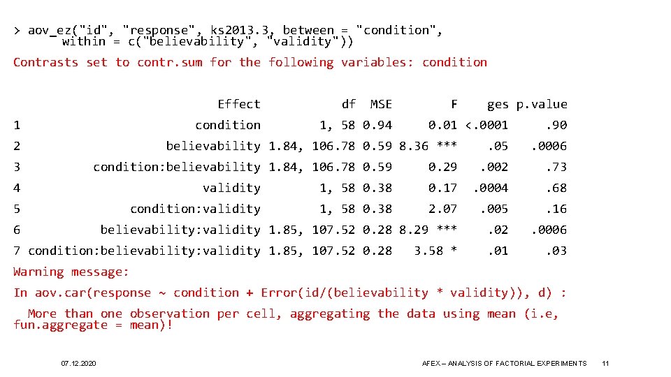
> aov_ez("id", "response", ks 2013. 3, between = "condition", within = c("believability", "validity")) Contrasts set to contr. sum for the following variables: condition Effect 1 condition 2 3 df MSE 1, 58 0. 94 F 0. 01 <. 0001 believability 1. 84, 106. 78 0. 59 8. 36 *** condition: believability 1. 84, 106. 78 0. 59 ges p. value. 90 . 05 . 0006 0. 29 . 002 . 73 4 validity 1, 58 0. 38 0. 17 . 0004 . 68 5 condition: validity 1, 58 0. 38 2. 07 . 005 . 16 believability: validity 1. 85, 107. 52 0. 28 8. 29 *** . 02 . 0006 . 01 . 03 6 7 condition: believability: validity 1. 85, 107. 52 0. 28 3. 58 * Warning message: In aov. car(response ~ condition + Error(id/(believability * validity)), d) : More than one observation per cell, aggregating the data using mean (i. e, fun. aggregate = mean)! 07. 12. 2020 AFEX – ANALYSIS OF FACTORIAL EXPERIMENTS 11

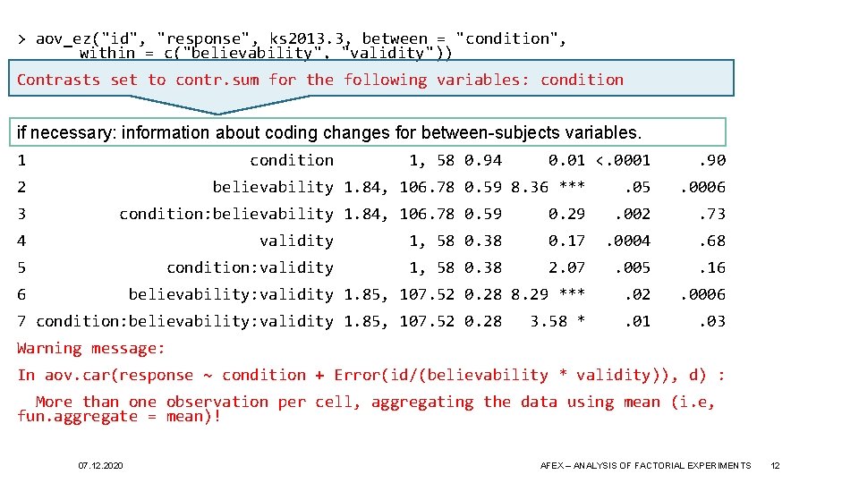
> aov_ez("id", "response", ks 2013. 3, between = "condition", within = c("believability", "validity")) Contrasts set to contr. sum for the following variables: condition if necessary: information about coding changes for between-subjects variables. Effect df MSE F ges p. value 1 condition 2 3 1, 58 0. 94 0. 01 <. 0001 believability 1. 84, 106. 78 0. 59 8. 36 *** condition: believability 1. 84, 106. 78 0. 59 . 90 . 05 . 0006 0. 29 . 002 . 73 4 validity 1, 58 0. 38 0. 17 . 0004 . 68 5 condition: validity 1, 58 0. 38 2. 07 . 005 . 16 believability: validity 1. 85, 107. 52 0. 28 8. 29 *** . 02 . 0006 . 01 . 03 6 7 condition: believability: validity 1. 85, 107. 52 0. 28 3. 58 * Warning message: In aov. car(response ~ condition + Error(id/(believability * validity)), d) : More than one observation per cell, aggregating the data using mean (i. e, fun. aggregate = mean)! 07. 12. 2020 AFEX – ANALYSIS OF FACTORIAL EXPERIMENTS 12

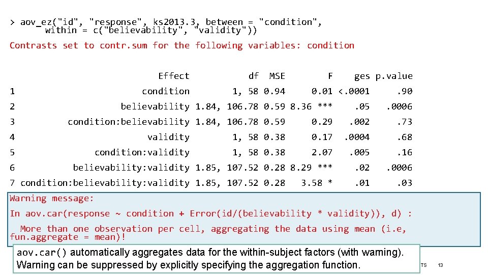
> aov_ez("id", "response", ks 2013. 3, between = "condition", within = c("believability", "validity")) Contrasts set to contr. sum for the following variables: condition Effect 1 condition 2 3 df MSE 1, 58 0. 94 F 0. 01 <. 0001 believability 1. 84, 106. 78 0. 59 8. 36 *** condition: believability 1. 84, 106. 78 0. 59 ges p. value. 90 . 05 . 0006 0. 29 . 002 . 73 4 validity 1, 58 0. 38 0. 17 . 0004 . 68 5 condition: validity 1, 58 0. 38 2. 07 . 005 . 16 believability: validity 1. 85, 107. 52 0. 28 8. 29 *** . 02 . 0006 . 01 . 03 6 7 condition: believability: validity 1. 85, 107. 52 0. 28 3. 58 * Warning message: In aov. car(response ~ condition + Error(id/(believability * validity)), d) : More than one observation per cell, aggregating the data using mean (i. e, fun. aggregate = mean)! aov. car() automatically aggregates data for the within-subject factors (with warning). 07. 12. 2020 AFEX –function. ANALYSIS OF FACTORIAL EXPERIMENTS Warning can be suppressed by explicitly specifying the aggregation 13

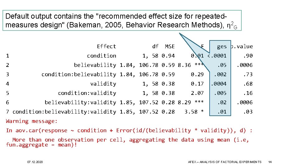
> aov_ez("id", "response", ks 2013. 3, between = "condition", Default output=contains the "recommended effect size for repeatedwithin c("believability", "validity")) measures design" (Bakeman, Behaviorvariables: Researchcondition Methods), η 2 G Contrasts set to contr. sum for 2005, the following Effect 1 condition 2 3 df MSE 1, 58 0. 94 F 0. 01 <. 0001 believability 1. 84, 106. 78 0. 59 8. 36 *** condition: believability 1. 84, 106. 78 0. 59 ges p. value. 90 . 05 . 0006 0. 29 . 002 . 73 4 validity 1, 58 0. 38 0. 17 . 0004 . 68 5 condition: validity 1, 58 0. 38 2. 07 . 005 . 16 believability: validity 1. 85, 107. 52 0. 28 8. 29 *** . 02 . 0006 . 01 . 03 6 7 condition: believability: validity 1. 85, 107. 52 0. 28 3. 58 * Warning message: In aov. car(response ~ condition + Error(id/(believability * validity)), d) : More than one observation per cell, aggregating the data using mean (i. e, fun. aggregate = mean)! 07. 12. 2020 AFEX – ANALYSIS OF FACTORIAL EXPERIMENTS 14

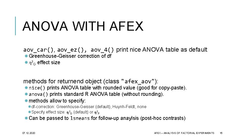
ANOVA WITH AFEX aov_car(), aov_ez(), aov_4() print nice ANOVA table as default Greenhouse-Geisser correction of df η 2 G effect size methods for returnend object (class "afex_aov"): nice() prints ANOVA table with rounded value (good for copy-paste). anova() prints standard R ANOVA table (without rounding). methods allow to specify: df-correction: Greenhouse-Geisser (default), Huynh-Feldt, none Specify effect size: η 2 G (default) or η 2 P Can be passed to lsmeans for follow-up anaylsis (post-hoc contrasts) 07. 12. 2020 AFEX – ANALYSIS OF FACTORIAL EXPERIMENTS 15

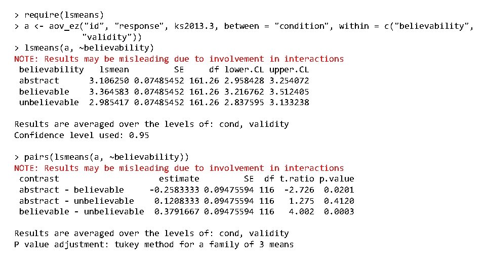
> require(lsmeans) > a <- aov_ez("id", "response", ks 2013. 3, between = "condition", within = c("believability", "validity")) > lsmeans(a, ~believability) NOTE: Results may be misleading due to involvement in interactions believability lsmean SE df lower. CL upper. CL abstract 3. 106250 0. 07485452 161. 26 2. 958428 3. 254072 believable 3. 364583 0. 07485452 161. 26 3. 216762 3. 512405 unbelievable 2. 985417 0. 07485452 161. 26 2. 837595 3. 133238 Results are averaged over the levels of: cond, validity Confidence level used: 0. 95 > pairs(lsmeans(a, ~believability)) NOTE: Results may be misleading due to involvement in interactions contrast estimate SE df t. ratio p. value abstract - believable -0. 2583333 0. 09475594 116 -2. 726 0. 0201 abstract - unbelievable 0. 1208333 0. 09475594 116 1. 275 0. 4120 believable - unbelievable 0. 3791667 0. 09475594 116 4. 002 0. 0003 Results are averaged over the levels of: cond, validity P value adjustment: tukey method for a family of 3 means

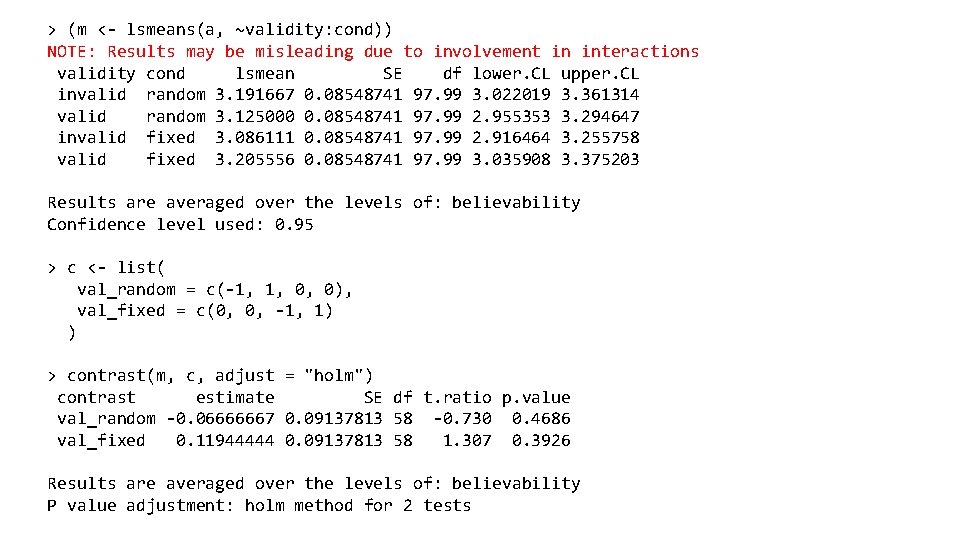
> (m <- lsmeans(a, ~validity: cond)) NOTE: Results may be misleading due to involvement in interactions validity cond lsmean SE df lower. CL upper. CL invalid random 3. 191667 0. 08548741 97. 99 3. 022019 3. 361314 valid random 3. 125000 0. 08548741 97. 99 2. 955353 3. 294647 invalid fixed 3. 086111 0. 08548741 97. 99 2. 916464 3. 255758 valid fixed 3. 205556 0. 08548741 97. 99 3. 035908 3. 375203 Results are averaged over the levels of: believability Confidence level used: 0. 95 > c <- list( val_random = c(-1, 1, 0, 0), val_fixed = c(0, 0, -1, 1) ) > contrast(m, c, adjust = "holm") contrast estimate SE df t. ratio p. value val_random -0. 06666667 0. 09137813 58 -0. 730 0. 4686 val_fixed 0. 11944444 0. 09137813 58 1. 307 0. 3926 Results are averaged over the levels of: believability P value adjustment: holm method for 2 tests

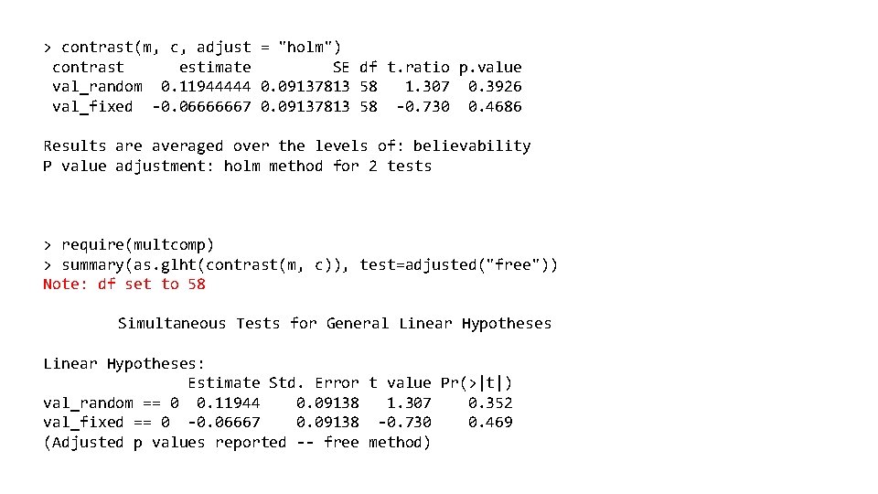
> contrast(m, c, adjust = "holm") contrast estimate SE df t. ratio p. value val_random 0. 11944444 0. 09137813 58 1. 307 0. 3926 val_fixed -0. 06666667 0. 09137813 58 -0. 730 0. 4686 Results are averaged over the levels of: believability P value adjustment: holm method for 2 tests > require(multcomp) > summary(as. glht(contrast(m, c)), test=adjusted("free")) Note: df set to 58 Simultaneous Tests for General Linear Hypotheses: Estimate Std. Error t value Pr(>|t|) val_random == 0 0. 11944 0. 09138 1. 307 0. 352 val_fixed == 0 -0. 06667 0. 09138 -0. 730 0. 469 (Adjusted p values reported -- free method)

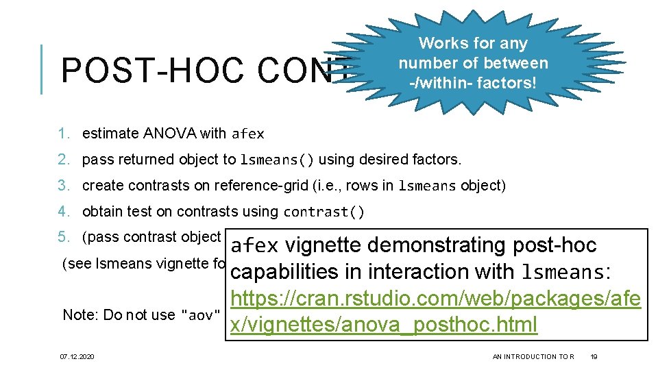
Works for any number of between -/within- factors! POST-HOC CONTRASTS 1. estimate ANOVA with afex 2. pass returned object to lsmeans() using desired factors. 3. create contrasts on reference-grid (i. e. , rows in lsmeans object) 4. obtain test on contrasts using contrast() 5. (pass contrast object to multcomp for advanced p-value corrections) afex vignette demonstrating post-hoc (see lsmeans vignette for more details) capabilities in interaction with lsmeans: https: //cran. rstudio. com/web/packages/afe Note: Do not use "aov" ANOVA for assessing effects! x/vignettes/anova_posthoc. html 07. 12. 2020 AN INTRODUCTION TO R 19

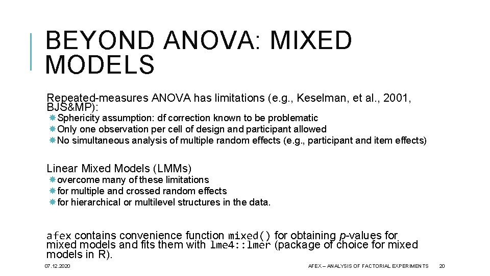
BEYOND ANOVA: MIXED MODELS Repeated-measures ANOVA has limitations (e. g. , Keselman, et al. , 2001, BJS&MP): Sphericity assumption: df correction known to be problematic Only one observation per cell of design and participant allowed No simultaneous analysis of multiple random effects (e. g. , participant and item effects) Linear Mixed Models (LMMs) overcome many of these limitations for multiple and crossed random effects for hierarchical or multilevel structures in the data. afex contains convenience function mixed() for obtaining p-values for mixed models and fits them with lme 4: : lmer (package of choice for mixed models in R). 07. 12. 2020 AFEX – ANALYSIS OF FACTORIAL EXPERIMENTS 20

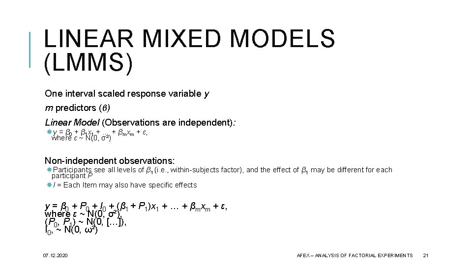
LINEAR MIXED MODELS (LMMS) One interval scaled response variable y m predictors (β) Linear Model (Observations are independent): y = β 0 + β 1 x 1 + … + βmxm + ε, where ε ~ N(0, σ²) Non-independent observations: Participants see all levels of β 1 (i. e. , within-subjects factor), and the effect of β 1 may be different for each participant P I = Each Item may also have specific effects y = β 0 + P 0 + I 0 + (β 1 + P 1)x 1 + … + βmxm + ε, where ε ~ N(0, σ²), (P 0, P 1) ~ N(0, […]), I 0, ~ N(0, ω²) 07. 12. 2020 AFEX – ANALYSIS OF FACTORIAL EXPERIMENTS 21

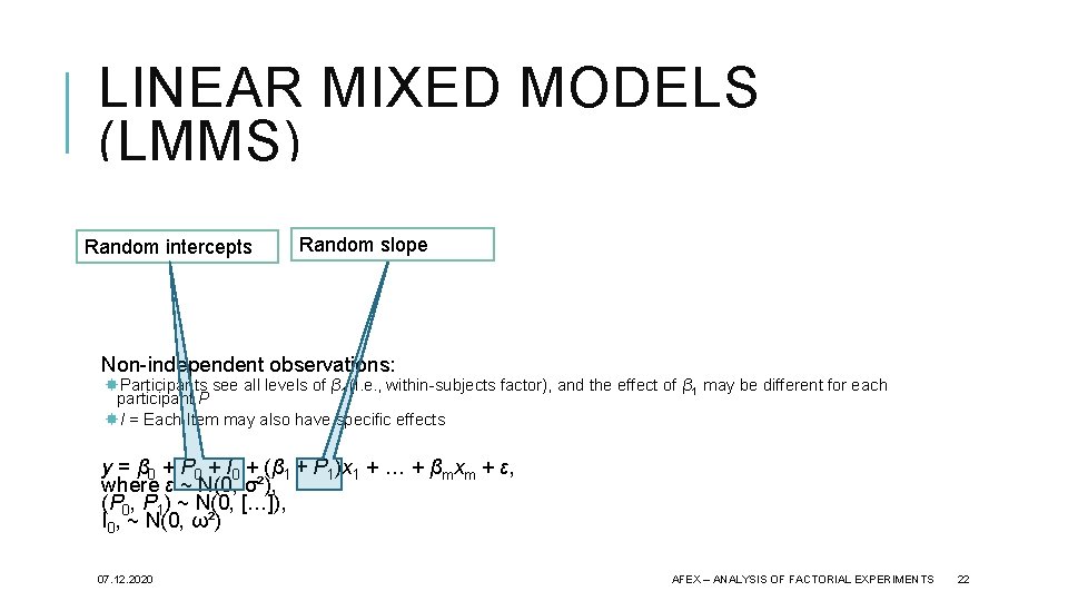
LINEAR MIXED MODELS (LMMS) One interval scaled response variable y m predictors (β) Random intercepts Random slope Linear Model (Observations are independent): y = β 0 + β 1 x 1 + … + βmxm + ε, where ε ~ N(0, σ²) Non-independent observations: Participants see all levels of β 1 (i. e. , within-subjects factor), and the effect of β 1 may be different for each participant P I = Each Item may also have specific effects y = β 0 + P 0 + I 0 + (β 1 + P 1)x 1 + … + βmxm + ε, where ε ~ N(0, σ²), (P 0, P 1) ~ N(0, […]), I 0, ~ N(0, ω²) 07. 12. 2020 AFEX – ANALYSIS OF FACTORIAL EXPERIMENTS 22

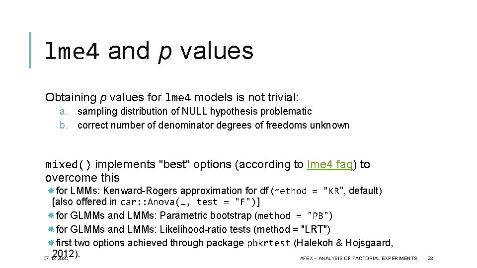
lme 4 and p values Obtaining p values for lme 4 models is not trivial: a. sampling distribution of NULL hypothesis problematic b. correct number of denominator degrees of freedoms unknown mixed() implements "best" options (according to lme 4 faq) to overcome this for LMMs: Kenward-Rogers approximation for df (method = "KR", default) [also offered in car: : Anova(…, test = "F")] for GLMMs and LMMs: Parametric bootstrap (method = "PB") for GLMMs and LMMs: Likelihood-ratio tests (method = "LRT") first two options achieved through package pbkrtest (Halekoh & Hojsgaard, 2012). 07. 12. 2020 AFEX – ANALYSIS OF FACTORIAL EXPERIMENTS 23

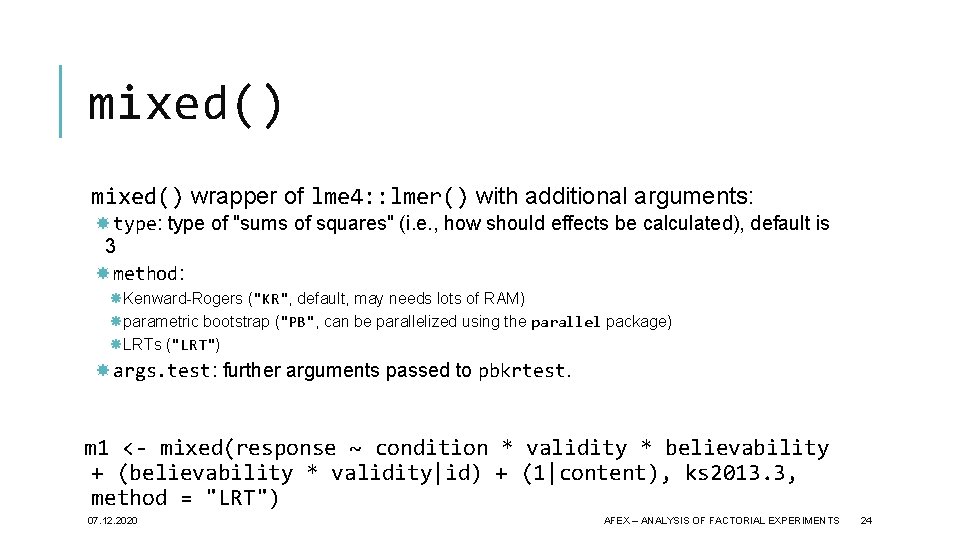
mixed() wrapper of lme 4: : lmer() with additional arguments: type: type of "sums of squares" (i. e. , how should effects be calculated), default is 3 method: Kenward-Rogers ("KR", default, may needs lots of RAM) parametric bootstrap ("PB", can be parallelized using the parallel package) LRTs ("LRT") args. test: further arguments passed to pbkrtest. m 1 <- mixed(response ~ condition * validity * believability + (believability * validity|id) + (1|content), ks 2013. 3, method = "LRT") 07. 12. 2020 AFEX – ANALYSIS OF FACTORIAL EXPERIMENTS 24

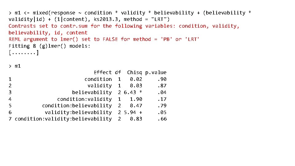
> m 1 <- mixed(response ~ condition * validity * believability + (believability * validity|id) + (1|content), ks 2013. 3, method = "LRT") Contrasts set to contr. sum for the following variables: condition, validity, believability, id, content REML argument to lmer() set to FALSE for method = 'PB' or 'LRT' Fitting 8 (g)lmer() models: [. . . . ] > m 1 1 2 3 4 5 6 7 Effect df Chisq p. value condition 1 0. 02. 90 validity 1 0. 03. 87 believability 2 6. 43 *. 04 condition: validity 1 1. 90. 17 condition: believability 2 0. 47. 79 validity: believability 2 5. 94 +. 05 condition: validity: believability 2 0. 83. 66

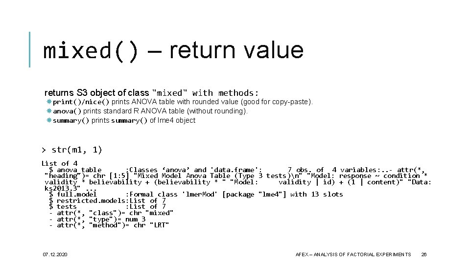
mixed() – return value returns S 3 object of class "mixed" with methods: print()/nice() prints ANOVA table with rounded value (good for copy-paste). anova() prints standard R ANOVA table (without rounding). summary() prints summary() of lme 4 object > str(m 1, 1) List of 4 $ anova_table : Classes ‘anova’ and 'data. frame': 7 obs. of 4 variables: . . - attr(*, "heading")= chr [1: 5] "Mixed Model Anova Table (Type 3 tests)n" "Model: response ~ condition * validity * believability + (believability * " "Model: validity | id) + (1 | content)" "Data: ks 2013. 3". . . $ full. model : Formal class 'lmer. Mod' [package "lme 4"] with 13 slots $ restricted. models: List of 7 $ tests : List of 7 - attr(*, "class")= chr "mixed" - attr(*, "type")= num 3 - attr(*, "method")= chr "LRT" 07. 12. 2020 AFEX – ANALYSIS OF FACTORIAL EXPERIMENTS 26

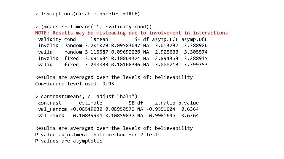
> lsm. options(disable. pbkrtest=TRUE) > (means <- lsmeans(m 1, ~validity: cond)) NOTE: Results may be misleading due to involvement in interactions validity cond lsmean SE df asymp. LCL asymp. UCL invalid random 3. 201079 0. 09583047 NA 3. 013232 3. 388926 valid random 3. 115587 0. 09692236 NA 2. 925600 3. 305574 invalid fixed 3. 091634 0. 10064324 NA 2. 894353 3. 288915 valid fixed 3. 200033 0. 10168346 NA 3. 000713 3. 399353 Results are averaged over the levels of: believability Confidence level used: 0. 95 > contrast(means, c, adjust="holm") contrast estimate SE df z. ratio p. value val_random -0. 08549232 0. 08950572 NA -0. 9551604 0. 6364 val_fixed 0. 10839904 0. 10859837 NA 0. 9981645 0. 6364 Results are averaged over the levels of: believability P value adjustment: holm method for 2 tests P values are asymptotic

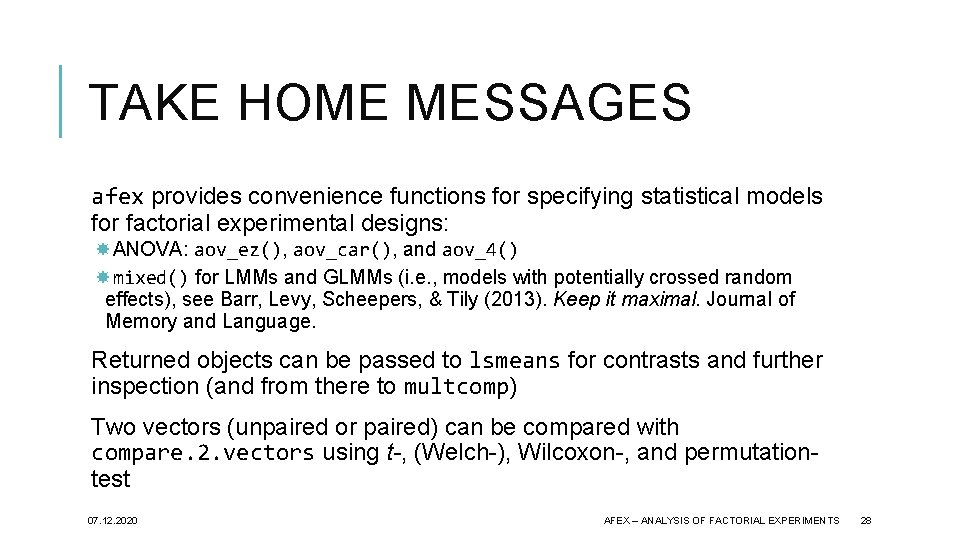
TAKE HOME MESSAGES afex provides convenience functions for specifying statistical models for factorial experimental designs: ANOVA: aov_ez(), aov_car(), and aov_4() mixed() for LMMs and GLMMs (i. e. , models with potentially crossed random effects), see Barr, Levy, Scheepers, & Tily (2013). Keep it maximal. Journal of Memory and Language. Returned objects can be passed to lsmeans for contrasts and further inspection (and from there to multcomp) Two vectors (unpaired or paired) can be compared with compare. 2. vectors using t-, (Welch-), Wilcoxon-, and permutationtest 07. 12. 2020 AFEX – ANALYSIS OF FACTORIAL EXPERIMENTS 28

THANK YOU FOR YOUR ATTENTION

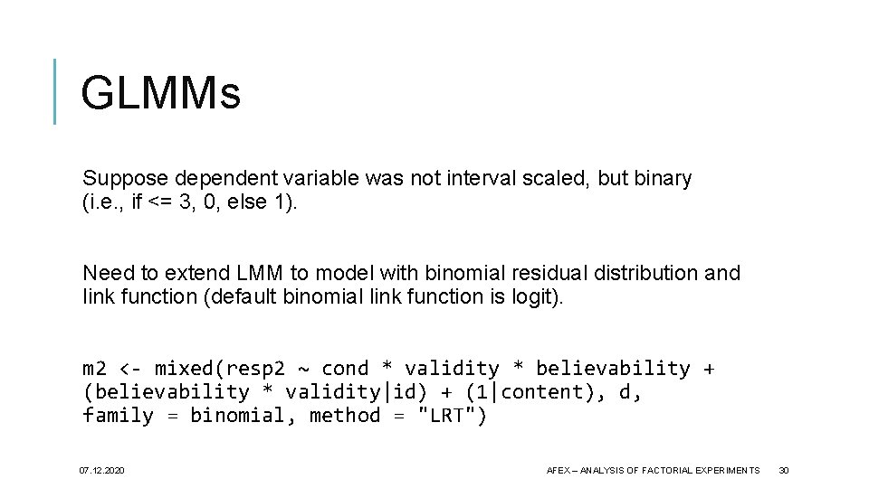
GLMMs Suppose dependent variable was not interval scaled, but binary (i. e. , if <= 3, 0, else 1). Need to extend LMM to model with binomial residual distribution and link function (default binomial link function is logit). m 2 <- mixed(resp 2 ~ cond * validity * believability + (believability * validity|id) + (1|content), d, family = binomial, method = "LRT") 07. 12. 2020 AFEX – ANALYSIS OF FACTORIAL EXPERIMENTS 30

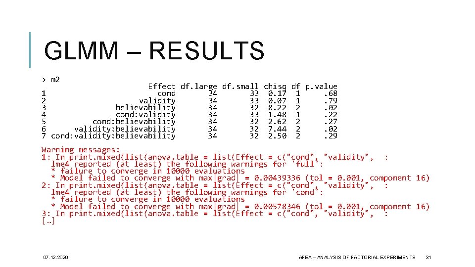
GLMM – RESULTS > m 2 Effect df. large df. small chisq df p. value 1 cond 34 33 0. 17 1. 68 2 validity 34 33 0. 07 1. 79 3 believability 34 32 8. 22 2. 02 4 cond: validity 34 33 1. 48 1. 22 5 cond: believability 34 32 2. 62 2. 27 6 validity: believability 34 32 7. 44 2. 02 7 cond: validity: believability 34 32 2. 50 2. 29 Warning messages: 1: In print. mixed(list(anova. table = list(Effect = c("cond", "validity", : lme 4 reported (at least) the following warnings for 'full': * failure to converge in 10000 evaluations * Model failed to converge with max|grad| = 0. 00439336 (tol = 0. 001, component 16) 2: In print. mixed(list(anova. table = list(Effect = c("cond", "validity", : lme 4 reported (at least) the following warnings for 'cond': * failure to converge in 10000 evaluations * Model failed to converge with max|grad| = 0. 00578346 (tol = 0. 001, component 16) 3: In print. mixed(list(anova. table = list(Effect = c("cond", "validity", : […] 07. 12. 2020 AFEX – ANALYSIS OF FACTORIAL EXPERIMENTS 31

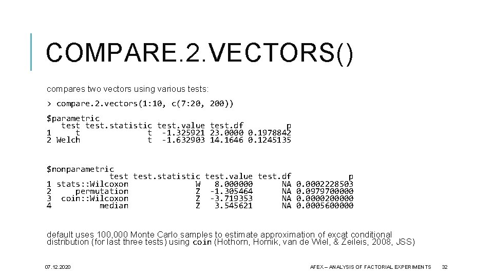
COMPARE. 2. VECTORS() compares two vectors using various tests: > compare. 2. vectors(1: 10, c(7: 20, 200)) $parametric test. statistic test. value test. df p 1 t t -1. 325921 23. 0000 0. 1978842 2 Welch t -1. 632903 14. 1646 0. 1245135 $nonparametric test. statistic test. value test. df p 1 stats: : Wilcoxon W 8. 000000 NA 0. 0002228503 2 permutation Z -1. 305464 NA 0. 0979700000 3 coin: : Wilcoxon Z -3. 719353 NA 0. 0000200000 4 median Z 3. 545621 NA 0. 0005600000 default uses 100, 000 Monte Carlo samples to estimate approximation of excat conditional distribution (for last three tests) using coin (Hothorn, Hornik, van de Wiel, & Zeileis, 2008, JSS) 07. 12. 2020 AFEX – ANALYSIS OF FACTORIAL EXPERIMENTS 32

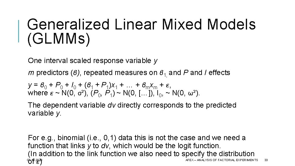
Generalized Linear Mixed Models (GLMMs) One interval scaled response variable y m predictors (β), repeated measures on β 1, and P and I effects y = β 0 + P 0 + I 0 + (β 1 + P 1)x 1 + … + βmxm + ε, where ε ~ N(0, σ²), (P 0, P 1) ~ N(0, […]), I 0, ~ N(0, ω²). The dependent variable dv directly corresponds to the predicted variable y. For e. g. , binomial (i. e. , 0, 1) data this is not the case and we need a function that links y to dv, which would be the logit function. (In addition to the link function we also need to specify the distribution 07. 12. 2020 AFEX – ANALYSIS OF FACTORIAL EXPERIMENTS of ε) 33

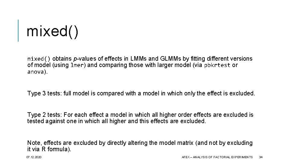
mixed() obtains p-values of effects in LMMs and GLMMs by fitting different versions of model (using lmer) and comparing those with larger model (via pbkrtest or anova). Type 3 tests: full model is compared with a model in which only the effect is excluded. Type 2 tests: For each effect a model in which all higher order effects are excluded is tested against one in which all higher and this effects are excluded. Note, effects are excluded by directly altering the model matrix (and not by excluding it via R formula). 07. 12. 2020 AFEX – ANALYSIS OF FACTORIAL EXPERIMENTS 34

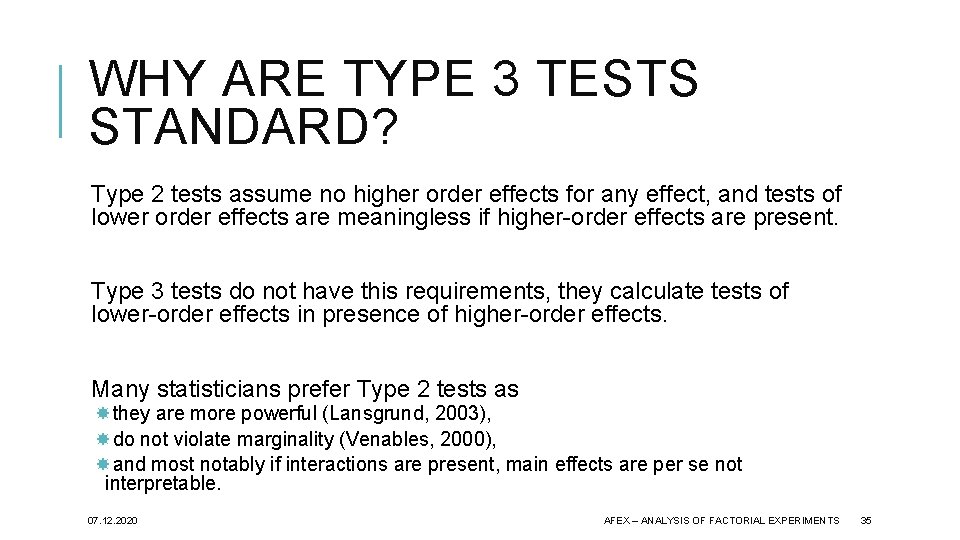
WHY ARE TYPE 3 TESTS STANDARD? Type 2 tests assume no higher order effects for any effect, and tests of lower order effects are meaningless if higher-order effects are present. Type 3 tests do not have this requirements, they calculate tests of lower-order effects in presence of higher-order effects. Many statisticians prefer Type 2 tests as they are more powerful (Lansgrund, 2003), do not violate marginality (Venables, 2000), and most notably if interactions are present, main effects are per se not interpretable. 07. 12. 2020 AFEX – ANALYSIS OF FACTORIAL EXPERIMENTS 35