afex Analysis of Factorial Experiments in R Henrik



- Slides: 33

afex – Analysis of Factorial Experiments in R Henrik Singmann

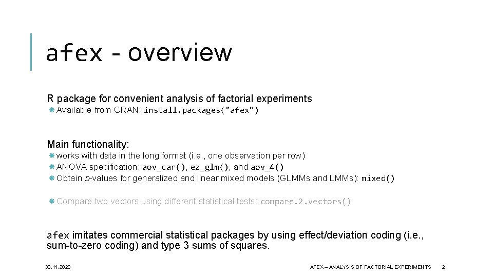
afex - overview R package for convenient analysis of factorial experiments Available from CRAN: install. packages("afex") Main functionality: works with data in the long format (i. e. , one observation per row) ANOVA specification: aov_car(), ez_glm(), and aov_4() Obtain p-values for generalized and linear mixed models (GLMMs and LMMs): mixed() Compare two vectors using different statistical tests: compare. 2. vectors() afex imitates commercial statistical packages by using effect/deviation coding (i. e. , sum-to-zero coding) and type 3 sums of squares. 30. 11. 2020 AFEX – ANALYSIS OF FACTORIAL EXPERIMENTS 2

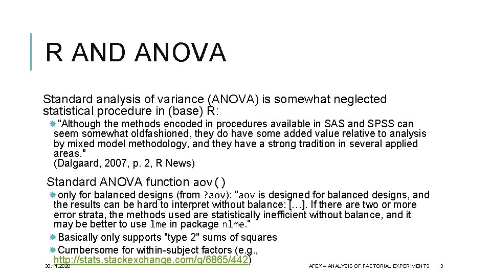
R AND ANOVA Standard analysis of variance (ANOVA) is somewhat neglected statistical procedure in (base) R: "Although the methods encoded in procedures available in SAS and SPSS can seem somewhat oldfashioned, they do have some added value relative to analysis by mixed model methodology, and they have a strong tradition in several applied areas. " (Dalgaard, 2007, p. 2, R News) Standard ANOVA function aov() only for balanced designs (from ? aov): "aov is designed for balanced designs, and the results can be hard to interpret without balance: […]. If there are two or more error strata, the methods used are statistically inefficient without balance, and it may be better to use lme in package nlme. " Basically only supports "type 2" sums of squares Cumbersome for within-subject factors (e. g. , http: //stats. stackexchange. com/q/6865/442) 30. 11. 2020 AFEX – ANALYSIS OF FACTORIAL EXPERIMENTS 3

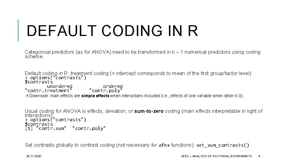
DEFAULT CODING IN R Categorical predictors (as for ANOVA) need to be transformed in k – 1 numerical predictors using coding scheme. Default coding in R: treatment coding (= intercept corresponds to mean of the first group/factor level): > options("contrasts") $contrasts unordered "contr. treatment" "contr. poly" Downside: main effects are simple effects when interactions included (i. e. , effects of one variable when other is 0). Usual coding for ANOVA is effects, deviation, or sum-to-zero coding (main effects interpretable in light of interactions): > options("contrasts") $contrasts [1] "contr. sum" "contr. poly" Set contrasts globally to contrast coding (not necessary for afex functions): set_sum_contrasts() 30. 11. 2020 AFEX – ANALYSIS OF FACTORIAL EXPERIMENTS 4

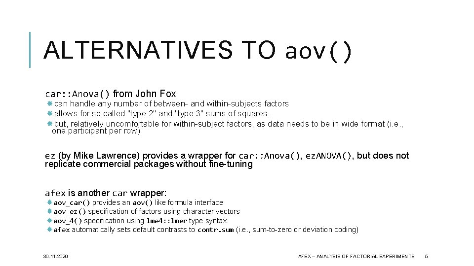
ALTERNATIVES TO aov() car: : Anova() from John Fox can handle any number of between- and within-subjects factors allows for so called "type 2" and "type 3" sums of squares. but, relatively uncomfortable for within-subject factors, as data needs to be in wide format (i. e. , one participant per row) ez (by Mike Lawrence) provides a wrapper for car: : Anova(), ez. ANOVA(), but does not replicate commercial packages without fine-tuning afex is another car wrapper: aov_car() provides an aov() like formula interface aov_ez() specification of factors using character vectors aov_4() specification using lme 4: : lmer type syntax. afex automatically sets default contrasts to contr. sum (i. e. , sum-to-zero or deviation coding) 30. 11. 2020 AFEX – ANALYSIS OF FACTORIAL EXPERIMENTS 5

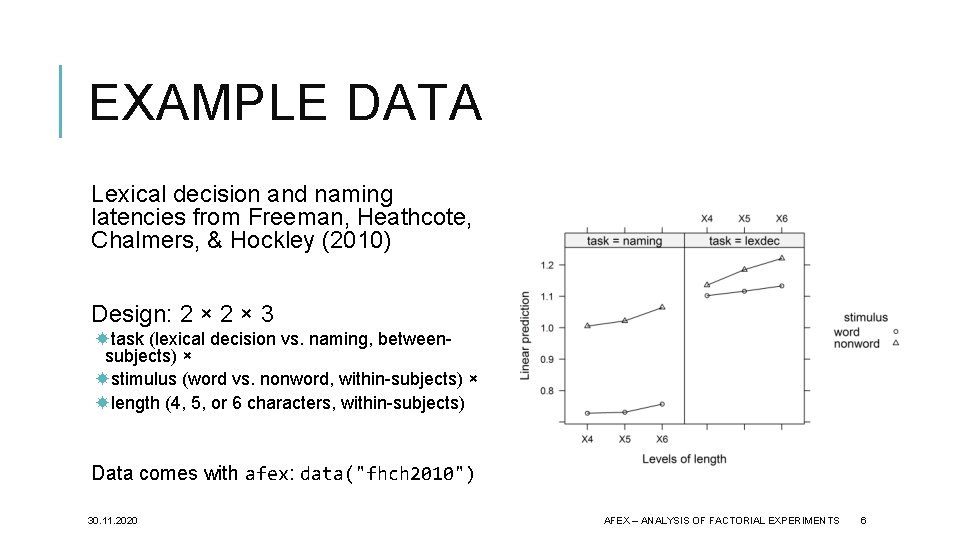
EXAMPLE DATA Lexical decision and naming latencies from Freeman, Heathcote, Chalmers, & Hockley (2010) Design: 2 × 3 task (lexical decision vs. naming, betweensubjects) × stimulus (word vs. nonword, within-subjects) × length (4, 5, or 6 characters, within-subjects) Data comes with afex: data("fhch 2010") 30. 11. 2020 AFEX – ANALYSIS OF FACTORIAL EXPERIMENTS 6

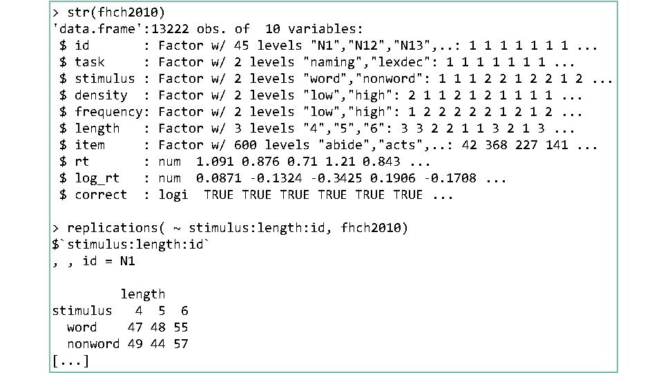
> str(fhch 2010) 'data. frame': 13222 obs. of 10 variables: $ id : Factor w/ 45 levels "N 1", "N 12", "N 13", . . : 1 1 1 1. . . $ task : Factor w/ 2 levels "naming", "lexdec": 1 1 1 1. . . $ stimulus : Factor w/ 2 levels "word", "nonword": 1 1 1 2 2 1 2. . . $ density : Factor w/ 2 levels "low", "high": 2 1 1. . . $ frequency: Factor w/ 2 levels "low", "high": 1 2 2 2 1 2. . . $ length : Factor w/ 3 levels "4", "5", "6": 3 3 2 2 1 1 3 2 1 3. . . $ item : Factor w/ 600 levels "abide", "acts", . . : 42 368 227 141. . . $ rt : num 1. 091 0. 876 0. 71 1. 21 0. 843. . . $ log_rt : num 0. 0871 -0. 1324 -0. 3425 0. 1906 -0. 1708. . . $ correct : logi TRUE TRUE. . . > replications( ~ stimulus: length: id, fhch 2010) $`stimulus: length: id` , , id = N 1 length stimulus 4 5 6 word 47 48 55 nonword 49 44 57 [. . . ] 7

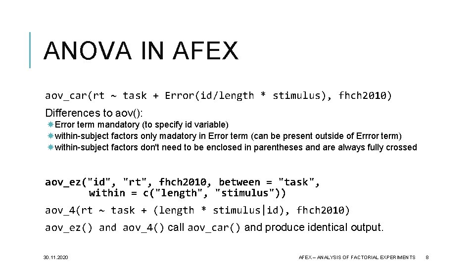
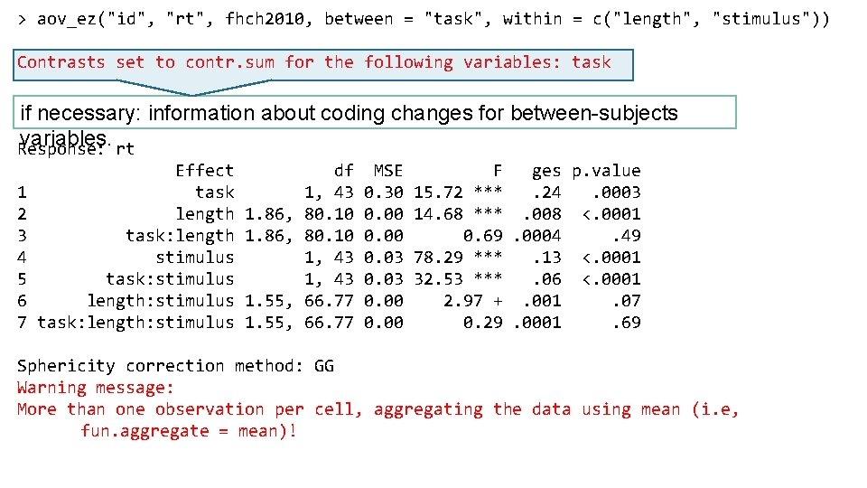
ANOVA IN AFEX aov_car(rt ~ task + Error(id/length * stimulus), fhch 2010) Differences to aov(): Error term mandatory (to specify id variable) within-subject factors only madatory in Error term (can be present outside of Errror term) within-subject factors don't need to be enclosed in parentheses and are always fully crossed aov_ez("id", "rt", fhch 2010, between = "task", within = c("length", "stimulus")) aov_4(rt ~ task + (length * stimulus|id), fhch 2010) aov_ez() and aov_4() call aov_car() and produce identical output. 30. 11. 2020 AFEX – ANALYSIS OF FACTORIAL EXPERIMENTS 8

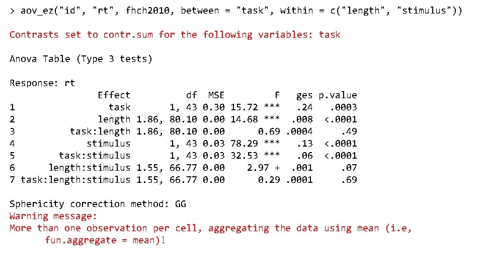
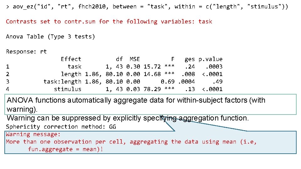
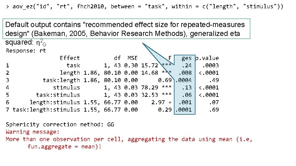
> aov_ez("id", "rt", fhch 2010, between = "task", within = c("length", "stimulus")) Contrasts set to contr. sum for the following variables: task Anova Table (Type 3 tests) Response: rt 1 2 3 4 5 6 7 Effect task length task: length stimulus task: stimulus length: stimulus task: length: stimulus 1. 86, 1. 55, df 1, 43 80. 10 1, 43 66. 77 MSE 0. 30 0. 00 0. 03 0. 00 F ges p. value 15. 72 ***. 24. 0003 14. 68 ***. 008 <. 0001 0. 69. 0004. 49 78. 29 ***. 13 <. 0001 32. 53 ***. 06 <. 0001 2. 97 +. 001. 07 0. 29. 0001. 69 Sphericity correction method: GG Warning message: More than one observation per cell, aggregating the data using mean (i. e, fun. aggregate = mean)!

> aov_ez("id", "rt", fhch 2010, between = "task", within = c("length", "stimulus")) Contrasts set to contr. sum for the following variables: task Anova Table (Type 3 tests) if necessary: information about coding changes for between-subjects variables. rt Response: 1 2 3 4 5 6 7 Effect task length task: length stimulus task: stimulus length: stimulus task: length: stimulus 1. 86, 1. 55, df 1, 43 80. 10 1, 43 66. 77 MSE 0. 30 0. 00 0. 03 0. 00 F ges p. value 15. 72 ***. 24. 0003 14. 68 ***. 008 <. 0001 0. 69. 0004. 49 78. 29 ***. 13 <. 0001 32. 53 ***. 06 <. 0001 2. 97 +. 001. 07 0. 29. 0001. 69 Sphericity correction method: GG Warning message: More than one observation per cell, aggregating the data using mean (i. e, fun. aggregate = mean)!

> aov_ez("id", "rt", fhch 2010, between = "task", within = c("length", "stimulus")) Contrasts set to contr. sum for the following variables: task Anova Table (Type 3 tests) Response: rt Effect df MSE F ges p. value 1 task 1, 43 0. 30 15. 72 ***. 24. 0003 2 length 1. 86, 80. 10 0. 00 14. 68 ***. 008 <. 0001 3 task: length 1. 86, 80. 10 0. 00 0. 69. 0004. 49 4 stimulus 1, 43 0. 03 78. 29 ***. 13 <. 0001 5 task: stimulus 1, 43 0. 03 32. 53 ***. 06 <. 0001 ANOVA functions automatically aggregate data for within-subject 6 length: stimulus 1. 55, 66. 77 0. 00 2. 97 +. 001. 07 7 warning). task: length: stimulus 1. 55, 66. 77 0. 00 0. 29. 0001. 69 factors (with Warning can be suppressed by explicitly specifying aggregation function. Sphericity correction method: GG Warning message: More than one observation per cell, aggregating the data using mean (i. e, fun. aggregate = mean)!

> aov_ez("id", "rt", fhch 2010, between = "task", within = c("length", "stimulus")) Contrasts set to contr. sum for the following variables: task Default output contains "recommended effect size for repeated-measures design" (Bakeman, Behavior Research Methods), generalized eta Anova Table (Type 32005, tests) squared: η 2 G Response: rt 1 2 3 4 5 6 7 Effect task length task: length stimulus task: stimulus length: stimulus task: length: stimulus 1. 86, 1. 55, df 1, 43 80. 10 1, 43 66. 77 MSE 0. 30 0. 00 0. 03 0. 00 F ges p. value 15. 72 ***. 24. 0003 14. 68 ***. 008 <. 0001 0. 69. 0004. 49 78. 29 ***. 13 <. 0001 32. 53 ***. 06 <. 0001 2. 97 +. 001. 07 0. 29. 0001. 69 Sphericity correction method: GG Warning message: More than one observation per cell, aggregating the data using mean (i. e, fun. aggregate = mean)!

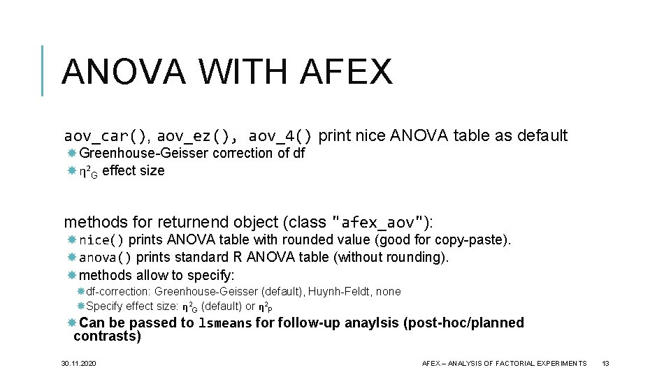
ANOVA WITH AFEX aov_car(), aov_ez(), aov_4() print nice ANOVA table as default Greenhouse-Geisser correction of df η 2 G effect size methods for returnend object (class "afex_aov"): nice() prints ANOVA table with rounded value (good for copy-paste). anova() prints standard R ANOVA table (without rounding). methods allow to specify: df-correction: Greenhouse-Geisser (default), Huynh-Feldt, none Specify effect size: η 2 G (default) or η 2 P Can be passed to lsmeans for follow-up anaylsis (post-hoc/planned contrasts) 30. 11. 2020 AFEX – ANALYSIS OF FACTORIAL EXPERIMENTS 13

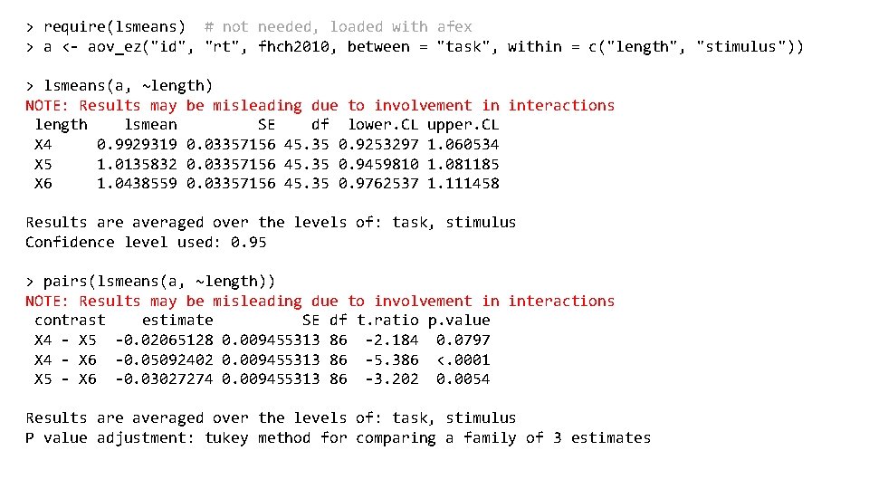
> require(lsmeans) # not needed, loaded with afex > a <- aov_ez("id", "rt", fhch 2010, between = "task", within = c("length", "stimulus")) > lsmeans(a, ~length) NOTE: Results may be misleading due to involvement in interactions length lsmean SE df lower. CL upper. CL X 4 0. 9929319 0. 03357156 45. 35 0. 9253297 1. 060534 X 5 1. 0135832 0. 03357156 45. 35 0. 9459810 1. 081185 X 6 1. 0438559 0. 03357156 45. 35 0. 9762537 1. 111458 Results are averaged over the levels of: task, stimulus Confidence level used: 0. 95 > pairs(lsmeans(a, ~length)) NOTE: Results may be misleading due to involvement in interactions contrast estimate SE df t. ratio p. value X 4 - X 5 -0. 02065128 0. 009455313 86 -2. 184 0. 0797 X 4 - X 6 -0. 05092402 0. 009455313 86 -5. 386 <. 0001 X 5 - X 6 -0. 03027274 0. 009455313 86 -3. 202 0. 0054 Results are averaged over the levels of: task, stimulus P value adjustment: tukey method for comparing a family of 3 estimates

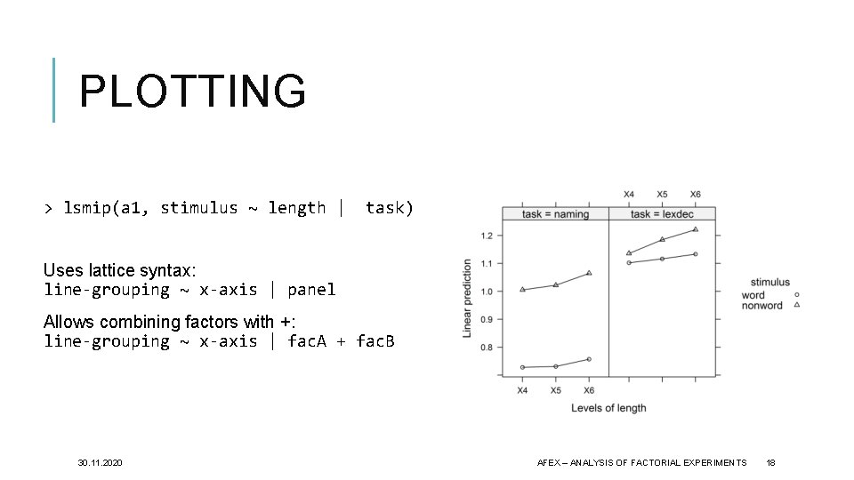
PLOTTING > lsmip(a 1, stimulus ~ length | task) Uses lattice syntax: line-grouping ~ x-axis | panel Allows combining factors with +: line-grouping ~ x-axis | fac. A + fac. B 30. 11. 2020 AFEX – ANALYSIS OF FACTORIAL EXPERIMENTS 15

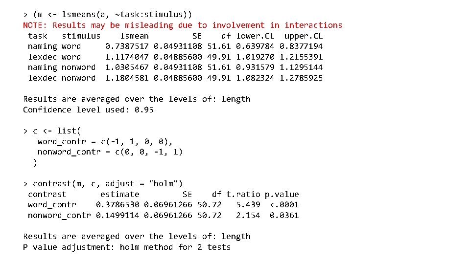
> (m <- lsmeans(a, ~task: stimulus)) NOTE: Results may be misleading due to involvement in interactions task stimulus lsmean SE df lower. CL upper. CL naming word 0. 7387517 0. 04931108 51. 61 0. 639784 0. 8377194 lexdec word 1. 1174047 0. 04885600 49. 91 1. 019270 1. 2155391 naming nonword 1. 0305467 0. 04931108 51. 61 0. 931579 1. 1295144 lexdec nonword 1. 1804581 0. 04885600 49. 91 1. 082324 1. 2785925 Results are averaged over the levels of: length Confidence level used: 0. 95 > c <- list( word_contr = c(-1, 1, 0, 0), nonword_contr = c(0, 0, -1, 1) ) > contrast(m, c, adjust = "holm") contrast estimate SE df t. ratio p. value word_contr 0. 3786530 0. 06961266 50. 72 5. 439 <. 0001 nonword_contr 0. 1499114 0. 06961266 50. 72 2. 154 0. 0361 Results are averaged over the levels of: length P value adjustment: holm method for 2 tests

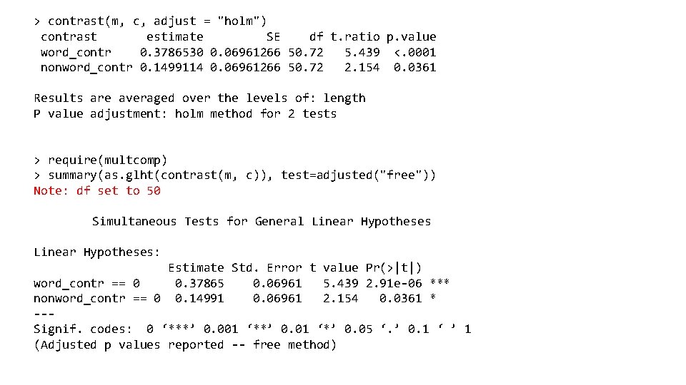
> contrast(m, c, adjust = "holm") contrast estimate SE df t. ratio p. value word_contr 0. 3786530 0. 06961266 50. 72 5. 439 <. 0001 nonword_contr 0. 1499114 0. 06961266 50. 72 2. 154 0. 0361 Results are averaged over the levels of: length P value adjustment: holm method for 2 tests > require(multcomp) > summary(as. glht(contrast(m, c)), test=adjusted("free")) Note: df set to 50 Simultaneous Tests for General Linear Hypotheses: Estimate Std. Error t value Pr(>|t|) word_contr == 0 0. 37865 0. 06961 5. 439 2. 91 e-06 *** nonword_contr == 0 0. 14991 0. 06961 2. 154 0. 0361 * --Signif. codes: 0 ‘***’ 0. 001 ‘**’ 0. 01 ‘*’ 0. 05 ‘. ’ 0. 1 ‘ ’ 1 (Adjusted p values reported -- free method)

PLOTTING > lsmip(a 1, stimulus ~ length | task) Uses lattice syntax: line-grouping ~ x-axis | panel Allows combining factors with +: line-grouping ~ x-axis | fac. A + fac. B 30. 11. 2020 AFEX – ANALYSIS OF FACTORIAL EXPERIMENTS 18

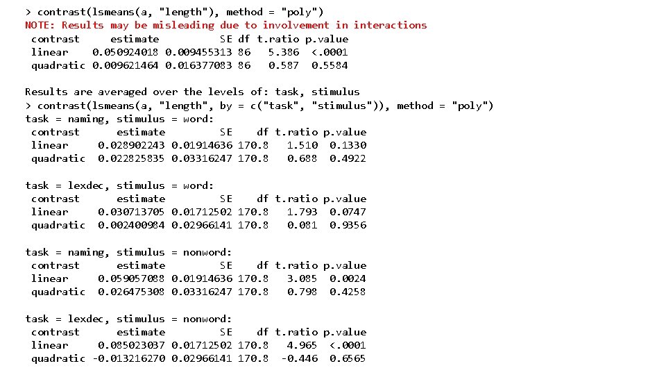
> contrast(lsmeans(a, "length"), method = "poly") NOTE: Results may be misleading due to involvement in interactions contrast estimate SE df t. ratio p. value linear 0. 050924018 0. 009455313 86 5. 386 <. 0001 quadratic 0. 009621464 0. 016377083 86 0. 587 0. 5584 Results are averaged over the levels of: task, stimulus > contrast(lsmeans(a, "length", by = c("task", "stimulus")), method = "poly") task = naming, stimulus = word: contrast estimate SE df t. ratio p. value linear 0. 028902243 0. 01914636 170. 8 1. 510 0. 1330 quadratic 0. 022825835 0. 03316247 170. 8 0. 688 0. 4922 task = lexdec, stimulus = word: contrast estimate SE df t. ratio p. value linear 0. 030713705 0. 01712502 170. 8 1. 793 0. 0747 quadratic 0. 002400984 0. 02966141 170. 8 0. 081 0. 9356 task = naming, stimulus = nonword: contrast estimate SE df t. ratio p. value linear 0. 059057088 0. 01914636 170. 8 3. 085 0. 0024 quadratic 0. 026475308 0. 03316247 170. 8 0. 798 0. 4258 task = lexdec, stimulus = nonword: contrast estimate SE df t. ratio p. value linear 0. 085023037 0. 01712502 170. 8 4. 965 <. 0001 quadratic -0. 013216270 0. 02966141 170. 8 -0. 446 0. 6565

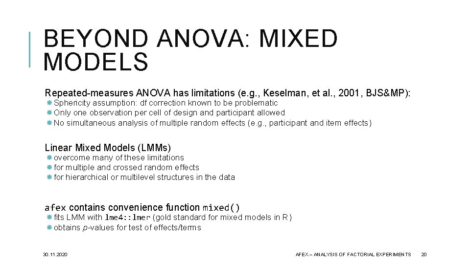
BEYOND ANOVA: MIXED MODELS Repeated-measures ANOVA has limitations (e. g. , Keselman, et al. , 2001, BJS&MP): Sphericity assumption: df correction known to be problematic Only one observation per cell of design and participant allowed No simultaneous analysis of multiple random effects (e. g. , participant and item effects) Linear Mixed Models (LMMs) overcome many of these limitations for multiple and crossed random effects for hierarchical or multilevel structures in the data afex contains convenience function mixed() fits LMM with lme 4: : lmer (gold standard for mixed models in R) obtains p-values for test of effects/terms 30. 11. 2020 AFEX – ANALYSIS OF FACTORIAL EXPERIMENTS 20

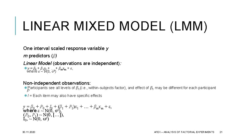
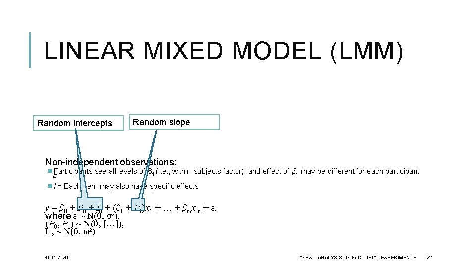
LINEAR MIXED MODEL (LMM) One interval scaled response variable y m predictors (β) Linear Model (observations are independent): y = β 0 + β 1 x 1 + … + βmxm + ε, where ε ~ N(0, σ²) Non-independent observations: Participants see all levels of β 1 (i. e. , within-subjects factor), and effect of β 1 may be different for each participant P I = Each item may also have specific effects y = β 0 + P 0 + I 0 + (β 1 + P 1)x 1 + … + βmxm + ε, where ε ~ N(0, σ²), (P 0, P 1) ~ N(0, […]), I 0, ~ N(0, ω²) 30. 11. 2020 AFEX – ANALYSIS OF FACTORIAL EXPERIMENTS 21

LINEAR MIXED MODEL (LMM) One interval scaled response variable y m predictors (β) Randomare slope Random Linear intercepts Model (Observations independent): y = β 0 + β 1 x 1 + … + βmxm + ε, where ε ~ N(0, σ²) Non-independent observations: Participants see all levels of β 1 (i. e. , within-subjects factor), and effect of β 1 may be different for each participant P I = Each Item may also have specific effects y = β 0 + P 0 + I 0 + (β 1 + P 1)x 1 + … + βmxm + ε, where ε ~ N(0, σ²), (P 0, P 1) ~ N(0, […]), I 0, ~ N(0, ω²) 30. 11. 2020 AFEX – ANALYSIS OF FACTORIAL EXPERIMENTS 22

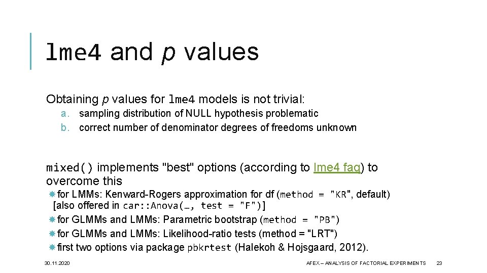
lme 4 and p values Obtaining p values for lme 4 models is not trivial: a. sampling distribution of NULL hypothesis problematic b. correct number of denominator degrees of freedoms unknown mixed() implements "best" options (according to lme 4 faq) to overcome this for LMMs: Kenward-Rogers approximation for df (method = "KR", default) [also offered in car: : Anova(…, test = "F")] for GLMMs and LMMs: Parametric bootstrap (method = "PB") for GLMMs and LMMs: Likelihood-ratio tests (method = "LRT") first two options via package pbkrtest (Halekoh & Hojsgaard, 2012). 30. 11. 2020 AFEX – ANALYSIS OF FACTORIAL EXPERIMENTS 23

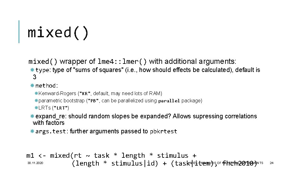
mixed() wrapper of lme 4: : lmer() with additional arguments: type: type of "sums of squares" (i. e. , how should effects be calculated), default is 3 method: Kenward-Rogers ("KR", default, may need lots of RAM) parametric bootstrap ("PB", can be parallelized using parallel package) LRTs ("LRT") expand_re: should random slopes be expanded? Allows supressing correlations with factors args. test: further arguments passed to pbkrtest m 1 <- mixed(rt ~ task * length * stimulus + 30. 11. 2020 AFEX – ANALYSIS OF FACTORIAL EXPERIMENTS (length * stimulus|id) + (task|item), fhch 2010) 24

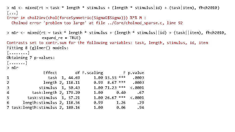
> m 1 <- mixed(rt ~ task * length * stimulus + (length * stimulus|id) + (task|item), fhch 2010) [. . . ] Error in chol 2 inv(chol(force. Symmetric(Sigma. G$Sigma))) %*% M : Cholmod error 'problem too large' at file. . /Core/cholmod_sparse. c, line 92 > m 1 r <- mixed(rt ~ task * length * stimulus + (length * stimulus||id) + (task||item), fhch 2010, expand_re = TRUE) Contrasts set to contr. sum for the following variables: task, length, stimulus, id, item Fitting 8 (g)lmer() models: [. . . . ] Obtaining 7 p-values: [. . . . ] > m 1 r Effect df F. scaling F p. value 1 task 1, 44. 69 1. 00 15. 55 ***. 0003 2 length 2, 118. 11 0. 99 8. 67 ***. 0003 3 stimulus 1, 50. 43 1. 00 71. 23 *** <. 0001 4 task: length 2, 179. 20 1. 00 0. 40. 67 5 task: stimulus 1, 57. 21 1. 00 26. 67 *** <. 0001 6 length: stimulus 2, 118. 56 0. 99 1. 26. 29 7 task: length: stimulus 2, 180. 16 1. 00 0. 06. 94

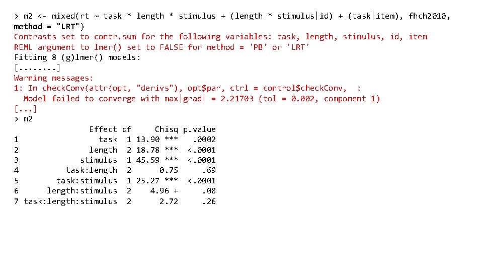
> m 2 <- mixed(rt ~ task * length * stimulus + (length * stimulus|id) + (task|item), fhch 2010, method = "LRT") Contrasts set to contr. sum for the following variables: task, length, stimulus, id, item REML argument to lmer() set to FALSE for method = 'PB' or 'LRT' Fitting 8 (g)lmer() models: [. . . . ] Warning messages: 1: In check. Conv(attr(opt, "derivs"), opt$par, ctrl = control$check. Conv, : Model failed to converge with max|grad| = 2. 21703 (tol = 0. 002, component 1) [. . . ] > m 2 Effect df Chisq p. value 1 task 1 13. 90 ***. 0002 2 length 2 18. 78 *** <. 0001 3 stimulus 1 45. 59 *** <. 0001 4 task: length 2 0. 75. 69 5 task: stimulus 1 25. 27 *** <. 0001 6 length: stimulus 2 4. 96 +. 08 7 task: length: stimulus 2 2. 72. 26

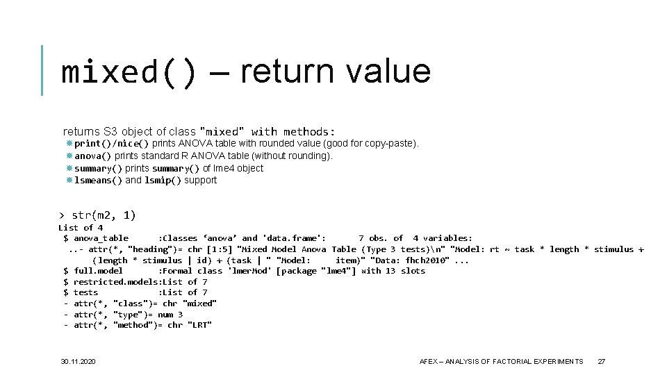
mixed() – return value returns S 3 object of class "mixed" with methods: print()/nice() prints ANOVA table with rounded value (good for copy-paste). anova() prints standard R ANOVA table (without rounding). summary() prints summary() of lme 4 object lsmeans() and lsmip() support > str(m 2, 1) List of 4 $ anova_table : Classes ‘anova’ and 'data. frame': 7 obs. of 4 variables: . . - attr(*, "heading")= chr [1: 5] "Mixed Model Anova Table (Type 3 tests)n" "Model: rt ~ task * length * stimulus + (length * stimulus | id) + (task | " "Model: item)" "Data: fhch 2010". . . $ full. model : Formal class 'lmer. Mod' [package "lme 4"] with 13 slots $ restricted. models: List of 7 $ tests : List of 7 - attr(*, "class")= chr "mixed" - attr(*, "type")= num 3 - attr(*, "method")= chr "LRT" 30. 11. 2020 AFEX – ANALYSIS OF FACTORIAL EXPERIMENTS 27

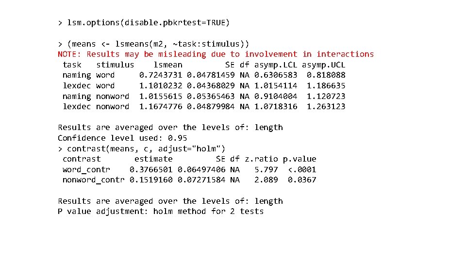
> lsm. options(disable. pbkrtest=TRUE) > (means <- lsmeans(m 2, ~task: stimulus)) NOTE: Results may be misleading due to involvement in interactions task stimulus lsmean SE df asymp. LCL asymp. UCL naming word 0. 7243731 0. 04781459 NA 0. 6306583 0. 818088 lexdec word 1. 1010232 0. 04368029 NA 1. 0154114 1. 186635 naming nonword 1. 0155615 0. 05365463 NA 0. 9104004 1. 120723 lexdec nonword 1. 1674776 0. 04879984 NA 1. 0718316 1. 263123 Results are averaged over the levels of: length Confidence level used: 0. 95 > contrast(means, c, adjust="holm") contrast estimate SE df z. ratio p. value word_contr 0. 3766501 0. 06497406 NA 5. 797 <. 0001 nonword_contr 0. 1519160 0. 07271584 NA 2. 089 0. 0367 Results are averaged over the levels of: length P value adjustment: holm method for 2 tests

TAKE HOME MESSAGES afex provides convenience functions for specifying statistical models for factorial experimental designs: ANOVA: aov_ez(), aov_car(), and aov_4() mixed() for LMMs and GLMMs (i. e. , models with potentially crossed random effects), see Barr, Levy, Scheepers, & Tily (2013). Keep it maximal. Journal of Memory and Language. Returned objects can be passed to lsmeans for contrasts and further inspection (and from there to multcomp) or to lsmip for plotting Two vectors (unpaired or paired) can be compared with compare. 2. vectors using t-, (Welch-), Wilcoxon-, and permutationtest 30. 11. 2020 AFEX – ANALYSIS OF FACTORIAL EXPERIMENTS 29

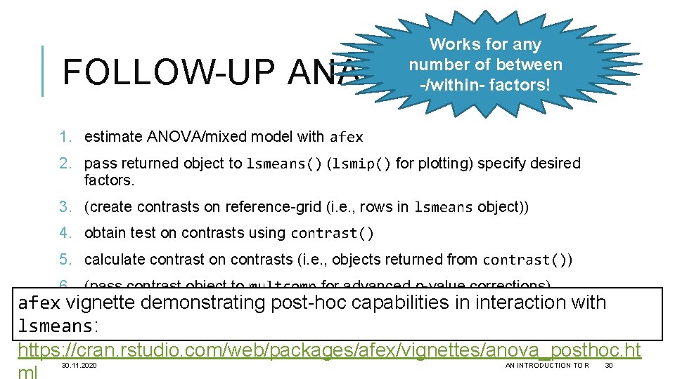
Works for any number of between -/within- factors! FOLLOW-UP ANALYSIS 1. estimate ANOVA/mixed model with afex 2. pass returned object to lsmeans() (lsmip() for plotting) specify desired factors. 3. (create contrasts on reference-grid (i. e. , rows in lsmeans object)) 4. obtain test on contrasts using contrast() 5. calculate contrast on contrasts (i. e. , objects returned from contrast()) 6. (pass contrast object to multcomp for advanced p-value corrections) afex (see vignette demonstrating post-hoc capabilities in interaction with lsmeans vignette for more details) lsmeans: https: //cran. rstudio. com/web/packages/afex/vignettes/anova_posthoc. ht 30. 11. 2020 AN INTRODUCTION TO R 30

THANK YOU FOR YOUR ATTENTION

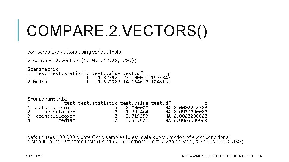
COMPARE. 2. VECTORS() compares two vectors using various tests: > compare. 2. vectors(1: 10, c(7: 20, 200)) $parametric test. statistic test. value test. df p 1 t t -1. 325921 23. 0000 0. 1978842 2 Welch t -1. 632903 14. 1646 0. 1245135 $nonparametric test. statistic test. value test. df p 1 stats: : Wilcoxon W 8. 000000 NA 0. 0002228503 2 permutation Z -1. 305464 NA 0. 0979700000 3 coin: : Wilcoxon Z -3. 719353 NA 0. 0000200000 4 median Z 3. 545621 NA 0. 0005600000 default uses 100, 000 Monte Carlo samples to estimate approximation of excat conditional distribution (for last three tests) using coin (Hothorn, Hornik, van de Wiel, & Zeileis, 2008, JSS) 30. 11. 2020 AFEX – ANALYSIS OF FACTORIAL EXPERIMENTS 32

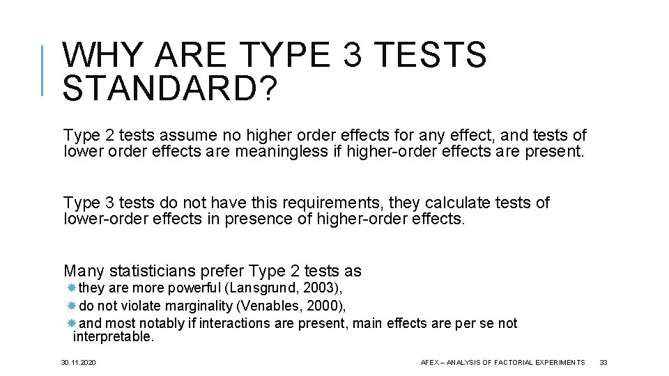
WHY ARE TYPE 3 TESTS STANDARD? Type 2 tests assume no higher order effects for any effect, and tests of lower order effects are meaningless if higher-order effects are present. Type 3 tests do not have this requirements, they calculate tests of lower-order effects in presence of higher-order effects. Many statisticians prefer Type 2 tests as they are more powerful (Lansgrund, 2003), do not violate marginality (Venables, 2000), and most notably if interactions are present, main effects are per se not interpretable. 30. 11. 2020 AFEX – ANALYSIS OF FACTORIAL EXPERIMENTS 33