Aalto University School of Engineering Stochastic Methods in

Aalto University School of Engineering Stochastic Methods in Engineering Stochastic Processes and Statistical Treatment of Loads and Response

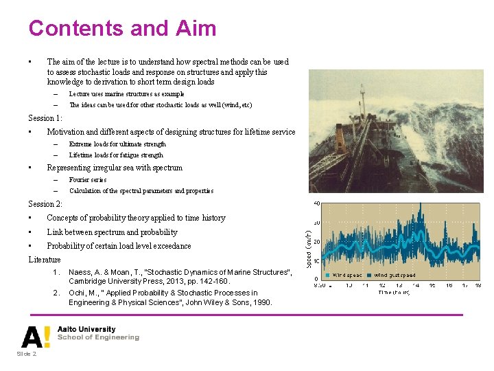
Contents and Aim • The aim of the lecture is to understand how spectral methods can be used to assess stochastic loads and response on structures and apply this knowledge to derivation to short term design loads – Lecture uses marine structures as example – The ideas can be used for other stochastic loads as well (wind, etc) Session 1: • • Motivation and different aspects of designing structures for lifetime service – Extreme loads for ultimate strength – Lifetime loads for fatigue strength Representing irregular sea with spectrum – Fourier series – Calculation of the spectral parameters and properties Session 2: • Concepts of probability theory applied to time history • Link between spectrum and probability • Probability of certain load level exceedance Literature 1. Naess, A. & Moan, T. , ”Stochastic Dynamics of Marine Structures”, Cambridge University Press, 2013, pp. 142 -160. 2. Slide 2 Ochi, M. , ” Applied Probability & Stochastic Processes in Engineering & Physical Sciences”, John Wiley & Sons, 1990.

Motivation Design of Structures • As engineers our duty is to: – – – • The process involves: – – – • Determination of loads (e. g. environmental such as wind, mechanical, thermal…) Defining response for given loads (e. g. stress, strain, displacement…) Checking if the strength is adequate (maximum stress, buckling etc) The lecture focuses on loads and assumptions made in the analysis: – – • Guarantee safety of structures/products we design Maximize the performance, e. g. wave energy absorption … Deterministic: load history is fully known (not valid in nature) Stochastic: we can only evaluate statistics related to the loads and responses, i. e. probability of exceedance of certain load level In order to FULLY understand the topic you are encouraged to take courses on Stochastic Processes

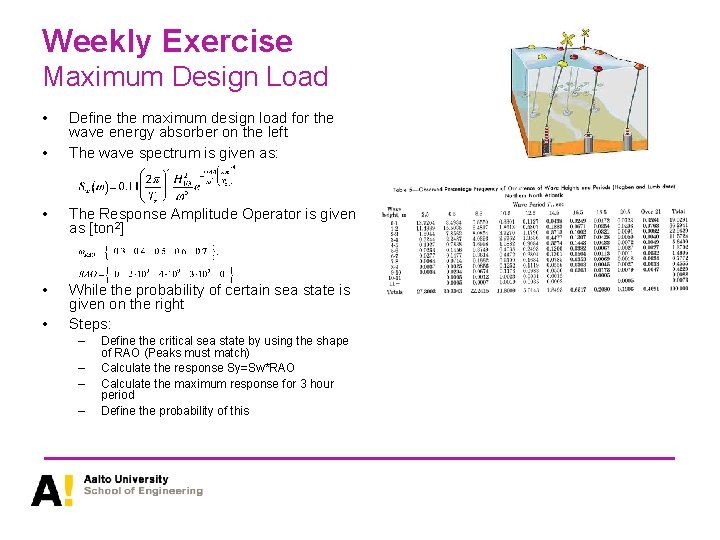
Weekly Exercise Maximum Design Load • • Define the maximum design load for the wave energy absorber on the left The wave spectrum is given as: • The Response Amplitude Operator is given as [ton 2] • While the probability of certain sea state is given on the right Steps: • – – Define the critical sea state by using the shape of RAO (Peaks must match) Calculate the response Sy=Sw*RAO Calculate the maximum response for 3 hour period Define the probability of this

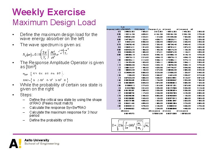
Weekly Exercise Maximum Design Load • • Define the maximum design load for the wave energy absorber on the left The wave spectrum is given as: • The Response Amplitude Operator is given as [ton 2] • While the probability of certain sea state is given on the right Steps: • – – Define the critical sea state by using the shape of RAO (Peaks must match) Calculate the response Sy=Sw*RAO Calculate the maximum response for 3 hour period Define the probability of this S_yy frequency (rad/s) (JONSWAP) RAO (Nm/m) Response S_xx m 1 (wave) m 1 (response) m 2 0, 5 3, 6583 E-203 7, 95 E-01 2, 91 E-203 1, 8291 E-203 1, 45 E-203 0, 55 1, 0221 E-138 4, 05 E-01 4, 14 E-139 5, 6218 E-139 2, 28 E-139 0, 6 5, 85391 E-98 2, 23 E-01 1, 31 E-98 3, 51235 E-98 7, 83 E-99 0, 65 3, 47726 E-71 1, 23 E-01 4, 28 E-72 2, 26022 E-71 2, 78 E-72 0, 7 5, 0001 E-53 6, 58 E-02 3, 29 E-54 3, 50007 E-53 2, 30 E-54 0, 75 2, 24979 E-40 3, 20 E-02 7, 20 E-42 1, 68734 E-40 5, 40 E-42 0, 8 2, 38451 E-31 1, 61 E-02 3, 84 E-33 1, 90761 E-31 3, 07 E-33 0, 85 8, 83432 E-25 1, 58 E-02 1, 40 E-26 7, 50917 E-25 1, 19 E-26 0, 9 6, 48408 E-20 1, 96 E-02 1, 27 E-21 5, 83567 E-20 1, 14 E-21 0, 95 2, 96388 E-16 2, 18 E-02 6, 46 E-18 2, 81569 E-16 6, 14 E-18 1 1, 82973 E-13 2, 21 E-02 4, 04 E-15 1, 82973 E-13 4, 04 E-15 1, 05 2, 60253 E-11 2, 11 E-02 5, 49 E-13 2, 73266 E-11 5, 77 E-13 1, 1 1, 24153 E-09 1, 93 E-02 2, 40 E-11 1, 36568 E-09 2, 64 E-11 1, 15 2, 59809 E-08 1, 70 E-02 4, 42 E-10 2, 9878 E-08 5, 08 E-10 1, 2 2, 89812 E-07 1, 45 E-02 4, 20 E-09 3, 47774 E-07 5, 04 E-09 1, 25 1, 98902 E-06 1, 19 E-02 2, 37 E-08 2, 48628 E-06 2, 96 E-08 1, 3 9, 34684 E-06 9, 88 E-03 9, 23 E-08 1, 21509 E-05 1, 20 E-07 1, 35 3, 26 E-05 7, 62 E-03 2, 48 E-07 4, 401 E-05 3, 35 E-07 1, 4 8, 97433 E-05 4, 88 E-03 4, 38 E-07 0, 000125641 6, 13 E-07 1, 45 0, 000204446 8, 50 E-03 1, 74 E-06 0, 000296447 2, 52 E-06 1, 5 0, 000399875 9, 94 E-03 3, 97 E-06 0, 000599812 5, 96 E-06 1, 55 0, 00069113 2, 77 E-03 1, 91 E-06 0, 001071251 2, 97 E-06 1, 6 0, 00107988 3, 01 E-03 3, 25 E-06 0, 001727809 5, 20 E-06 1, 65 0, 001553257 2, 06 E-03 3, 20 E-06 0, 002562874 5, 28 E-06 1, 7 0, 002086743 1, 17 E-03 2, 44 E-06 0, 003547464 4, 15 E-06 1, 75 0, 002649346 2, 49 E-03 6, 60 E-06 0, 004636355 1, 15 E-05 1, 8 0, 003209063 3, 43 E-03 1, 10 E-05 0, 005776313 1, 98 E-05 1, 85 0, 003737269 4, 09 E-03 1, 53 E-05 0, 006913947 2, 83 E-05 1, 9 0, 004211418 4, 65 E-03 1, 96 E-05 0, 008001694 3, 72 E-05 1, 95 0, 004616113 4, 75 E-03 2, 19 E-05 0, 00900142 4, 28 E-05 2 0, 004942923 4, 53 E-03 2, 24 E-05 0, 009885846 4, 48 E-05 m 0 (wave) m 0 (response) m 1 (wave) m 1 (response) 0, 001475773 5, 70581 E-06 0, 002710295 1, 05783 E-05 2, 50 E-02 2, 75 E-02 3, 00 E-02 3, 25 E-02 3, 50 E-02 3, 75 E-02 4, 00 E-02 4, 25 E-02 4, 50 E-02 4, 75 E-02 5, 00 E-02 5, 25 E-02 5, 50 E-02 5, 75 E-02 6, 00 E-02 6, 25 E-02 6, 49 E-02 6, 72 E-02 6, 87 E-02 7, 08 E-02 7, 20 E-02 5, 82 E-02 5, 13 E-02 2, 03 E-02 -6, 66 E-02 -5, 60 E-03 5, 80 E-03 7, 98 E-03 8, 96 E-03 2, 75 E-03 -9, 12 E-03

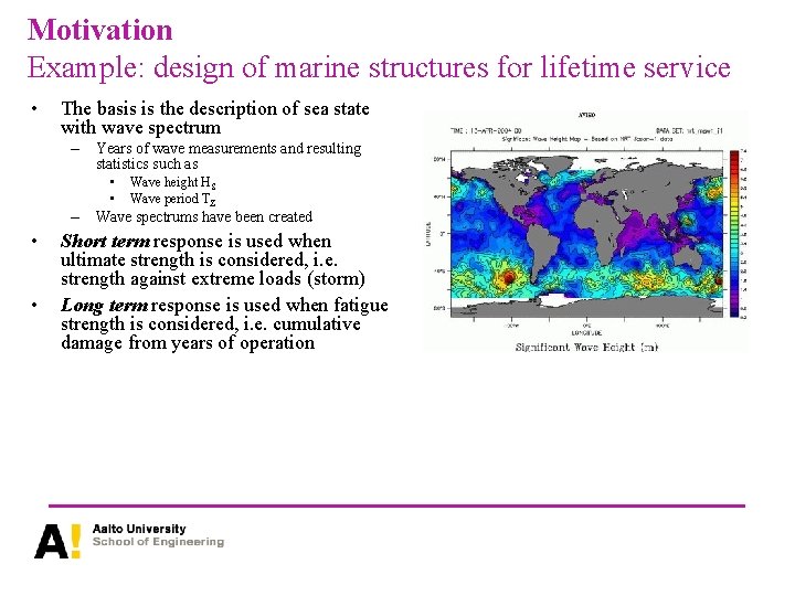
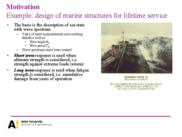
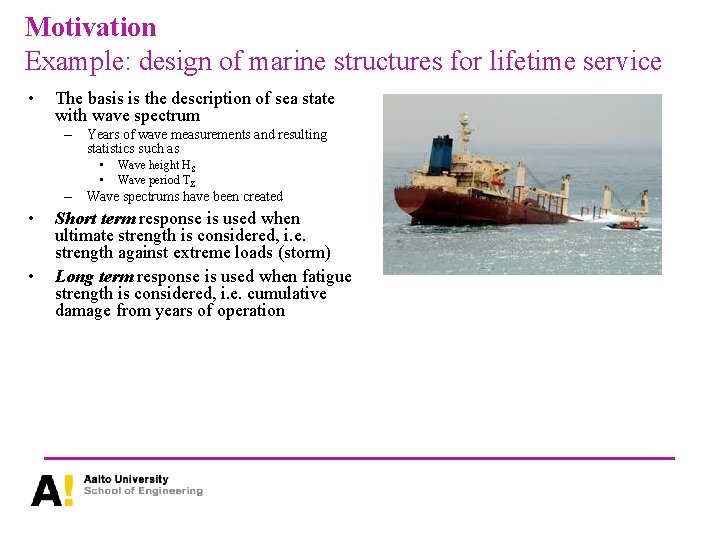
Motivation Example: design of marine structures for lifetime service • The basis is the description of sea state with wave spectrum – Years of wave measurements and resulting statistics such as • • Wave height HS Wave period TZ – Wave spectrums have been created • • Short term response is used when ultimate strength is considered, i. e. strength against extreme loads (storm) Long term response is used when fatigue strength is considered, i. e. cumulative damage from years of operation

Motivation Example: design of marine structures for lifetime service • The basis is the description of sea state with wave spectrum – Years of wave measurements and resulting statistics such as • • Wave height HS Wave period TZ – Wave spectrums have been created • • Short term response is used when ultimate strength is considered, i. e. strength against extreme loads (storm) Long term response is used when fatigue strength is considered, i. e. cumulative damage from years of operation

Motivation Example: design of marine structures for lifetime service • The basis is the description of sea state with wave spectrum – Years of wave measurements and resulting statistics such as • • Wave height HS Wave period TZ – Wave spectrums have been created • • Short term response is used when ultimate strength is considered, i. e. strength against extreme loads (storm) Long term response is used when fatigue strength is considered, i. e. cumulative damage from years of operation

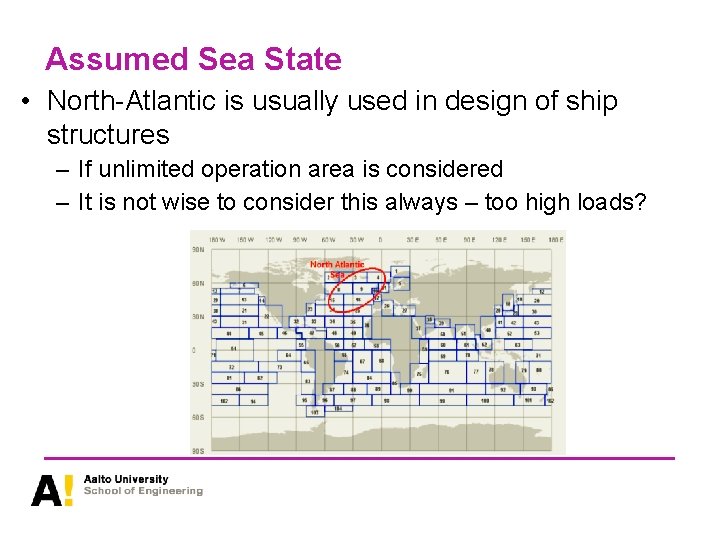
Assumed Sea State • North-Atlantic is usually used in design of ship structures – If unlimited operation area is considered – It is not wise to consider this always – too high loads?

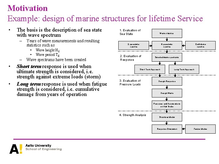
Motivation Example: design of marine structures for lifetime Service • The basis is the description of sea state with wave spectrum – Years of wave measurements and resulting statistics such as • • Wave height HS Wave period TZ – Wave spectrums have been created • • Short term response is used when ultimate strength is considered, i. e. strength against extreme loads (storm) Long term response is used when fatigue strength is considered, i. e. cumulative damage from years of operation 1. Evaluation of Sea State Wave statistics 2 -parameter spectra 6 -parameter spectra 2. Evaluation of Response Selected wave spectrums Short Term Approach 3. Evaluation of Pressure Loads Confidence spectra Long Term Approach Design Response Design Wave Pressures and Accelerations on Hull Girder 4. Strength Analysis Structural Model Response Evaluation Failure Modes

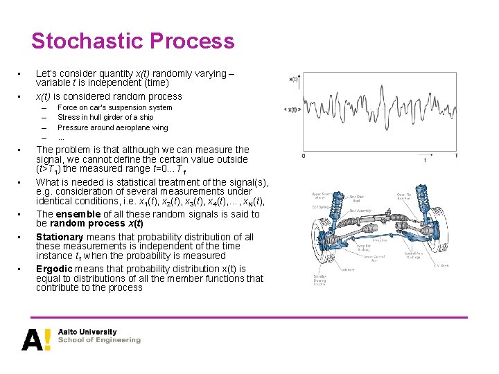
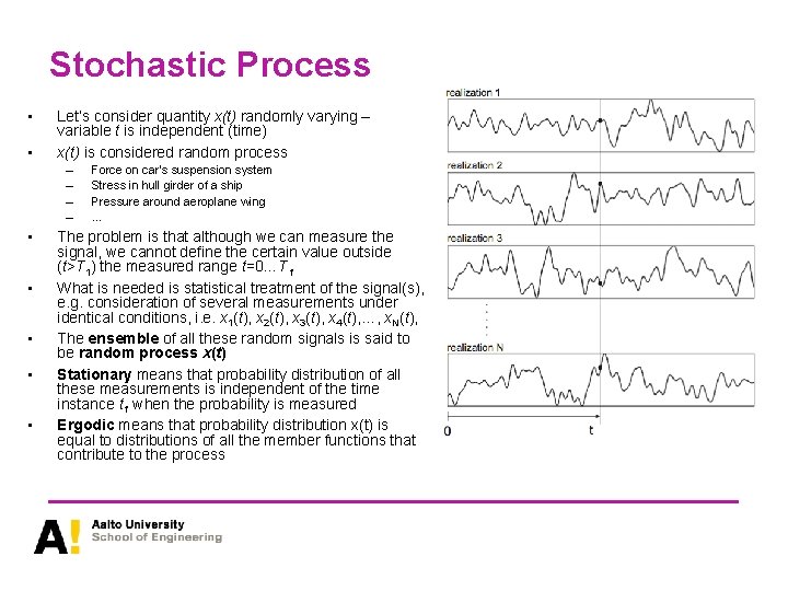
Stochastic Process • • Let’s consider quantity x(t) randomly varying – variable t is independent (time) x(t) is considered random process – – • • • Force on car’s suspension system Stress in hull girder of a ship Pressure around aeroplane wing … The problem is that although we can measure the signal, we cannot define the certain value outside (t>T 1) the measured range t=0…T 1 What is needed is statistical treatment of the signal(s), e. g. consideration of several measurements under identical conditions, i. e. x 1(t), x 2(t), x 3(t), x 4(t), …, x. N(t), The ensemble of all these random signals is said to be random process x(t) Stationary means that probability distribution of all these measurements is independent of the time instance t 1 when the probability is measured Ergodic means that probability distribution x(t) is equal to distributions of all the member functions that contribute to the process

Stochastic Process • • Let’s consider quantity x(t) randomly varying – variable t is independent (time) x(t) is considered random process – – • • • Force on car’s suspension system Stress in hull girder of a ship Pressure around aeroplane wing … The problem is that although we can measure the signal, we cannot define the certain value outside (t>T 1) the measured range t=0…T 1 What is needed is statistical treatment of the signal(s), e. g. consideration of several measurements under identical conditions, i. e. x 1(t), x 2(t), x 3(t), x 4(t), …, x. N(t), The ensemble of all these random signals is said to be random process x(t) Stationary means that probability distribution of all these measurements is independent of the time instance t 1 when the probability is measured Ergodic means that probability distribution x(t) is equal to distributions of all the member functions that contribute to the process

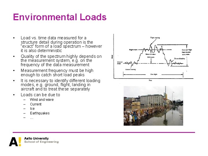
Environmental Loads • • • Load vs. time data measured for a structure detail during operation is the “exact” form of a load spectrum – however it is also deterministic Quality of the spectrum highly depends on the measurement system, e. g. on the frequency of the data measurement Measurement frequency must be high enough to catch short load peaks It is necessary to identify different loading modes, e. g. ground, flight, landing in aircraft and to treat these separately Loads can be due to – – – Wind and wave Current Ice Earthquakes …

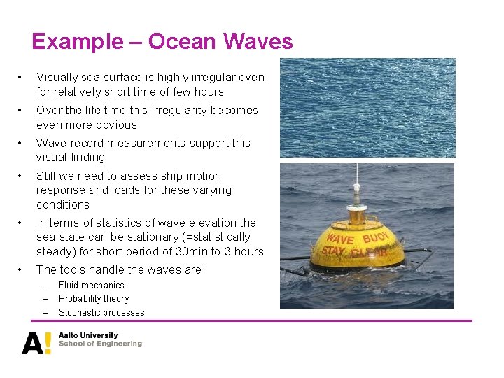
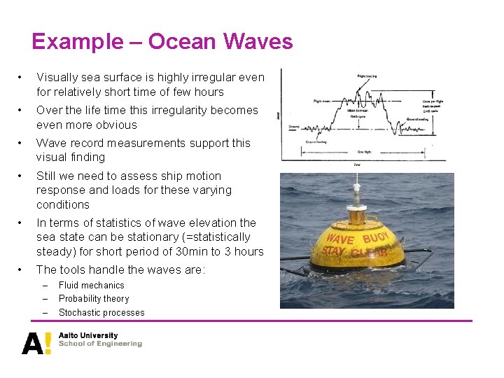
Example – Ocean Waves • Visually sea surface is highly irregular even for relatively short time of few hours • Over the life time this irregularity becomes even more obvious • Wave record measurements support this visual finding • Still we need to assess ship motion response and loads for these varying conditions • In terms of statistics of wave elevation the sea state can be stationary (=statistically steady) for short period of 30 min to 3 hours • The tools handle the waves are: – – – Fluid mechanics Probability theory Stochastic processes

Example – Ocean Waves • Visually sea surface is highly irregular even for relatively short time of few hours • Over the life time this irregularity becomes even more obvious • Wave record measurements support this visual finding • Still we need to assess ship motion response and loads for these varying conditions • In terms of statistics of wave elevation the sea state can be stationary (=statistically steady) for short period of 30 min to 3 hours • The tools handle the waves are: – – – Fluid mechanics Probability theory Stochastic processes

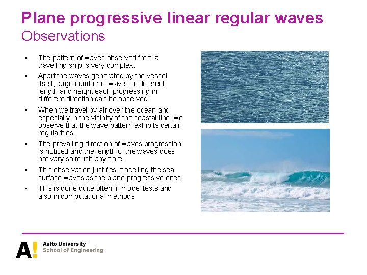
Plane progressive linear regular waves Observations • The pattern of waves observed from a travelling ship is very complex. • Apart the waves generated by the vessel itself, large number of waves of different length and height each progressing in different direction can be observed. • When we travel by air over the ocean and especially in the vicinity of the coastal line, we observe that the wave pattern exhibits certain regularities. • The prevailing direction of waves progression is noticed and the length of the waves does not vary so much anymore. • This observation justifies modelling the sea surface waves as the plane progressive ones. • This is done quite often in model tests and also in computational methods

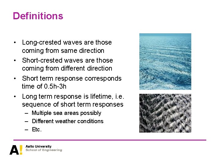
Definitions • Long-crested waves are those coming from same direction • Short-crested waves are those coming from different direction • Short term response corresponds time of 0. 5 h-3 h • Long term response is lifetime, i. e. sequence of short term responses – Multiple sea areas possibly – Different weather conditions – Etc.

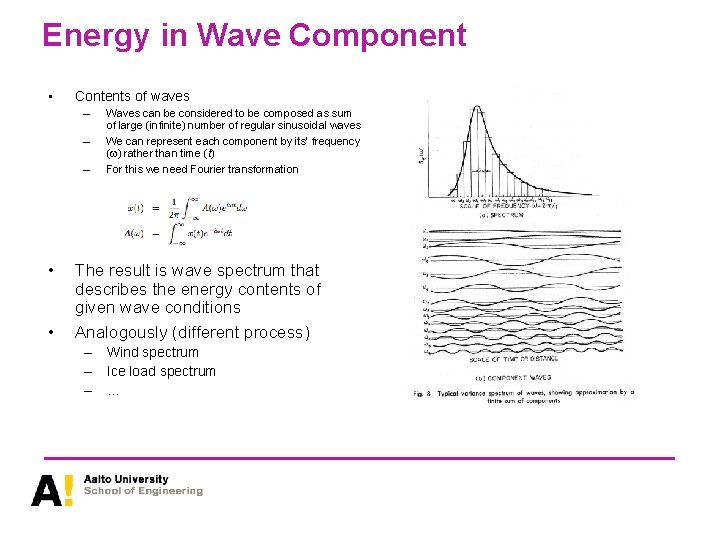
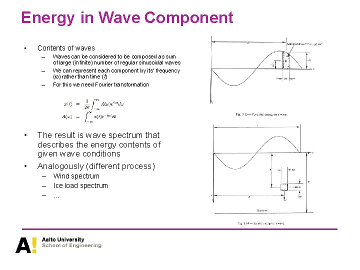
Energy in Wave Component • Contents of waves – – – • • Waves can be considered to be composed as sum of large (infinite) number of regular sinusoidal waves We can represent each component by its’ frequency (w) rather than time (t) For this we need Fourier transformation The result is wave spectrum that describes the energy contents of given wave conditions Analogously (different process) – Wind spectrum – Ice load spectrum – …

Energy in Wave Component • Contents of waves – – – • • Waves can be considered to be composed as sum of large (infinite) number of regular sinusoidal waves We can represent each component by its’ frequency (w) rather than time (t) For this we need Fourier transformation The result is wave spectrum that describes the energy contents of given wave conditions Analogously (different process) – Wind spectrum – Ice load spectrum – …

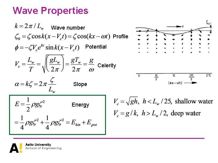
Wave Properties Wave number Profile Potential Celerity Slope Energy

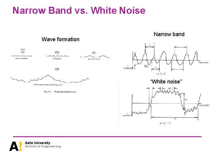
Narrow Band vs. White Noise Wave formation Narrow band “White noise”

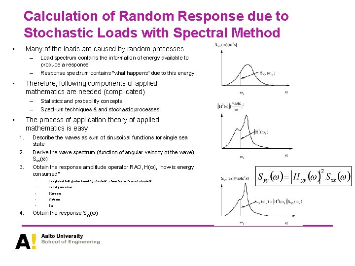
Calculation of Random Response due to Stochastic Loads with Spectral Method • Many of the loads are caused by random processes • – Load spectrum contains the information of energy available to produce a response – Response spectrum contains “what happens” due to this energy Therefore, following components of applied mathematics are needed (complicated) – – • Statistics and probability concepts Spectrum techniques & and stochastic processes The process of application theory of applied mathematics is easy 1. Describe the waves as sum of sinusoidal functions for single sea state 2. Derive the wave spectrum (function of angular velocity of the wave) Sxx(w) 3. Obtain the response amplitude operator RAO, H(w), “how is energy consumed” 4. • For global hull girder bending moment, shear force, torsion moment • Local pressures • Stresses • Motions • Etc Obtain the response Syy(w)

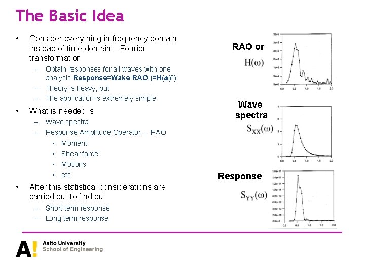
The Basic Idea • Consider everything in frequency domain instead of time domain – Fourier transformation – Obtain responses for all waves with one analysis Response=Wake*RAO (=H( )2) – Theory is heavy, but – The application is extremely simple • What is needed is – Wave spectra – Response Amplitude Operator – RAO • Moment • Shear force • Motions • etc • After this statistical considerations are carried out to find out – Short term response – Long term response RAO or Wave spectra Response

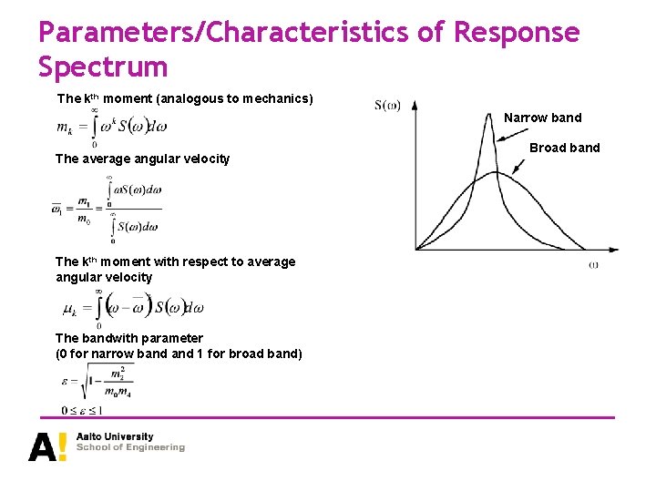
Parameters/Characteristics of Response Spectrum The kth moment (analogous to mechanics) Narrow band The average angular velocity The kth moment with respect to average angular velocity The bandwith parameter (0 for narrow band 1 for broad band) Broad band

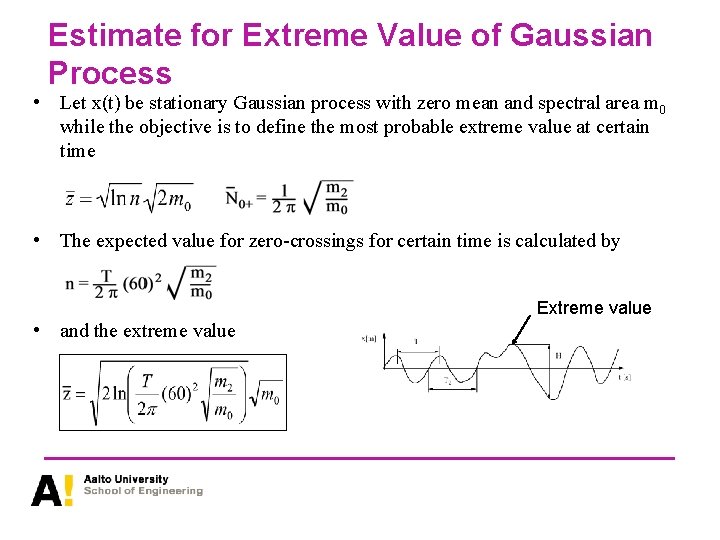
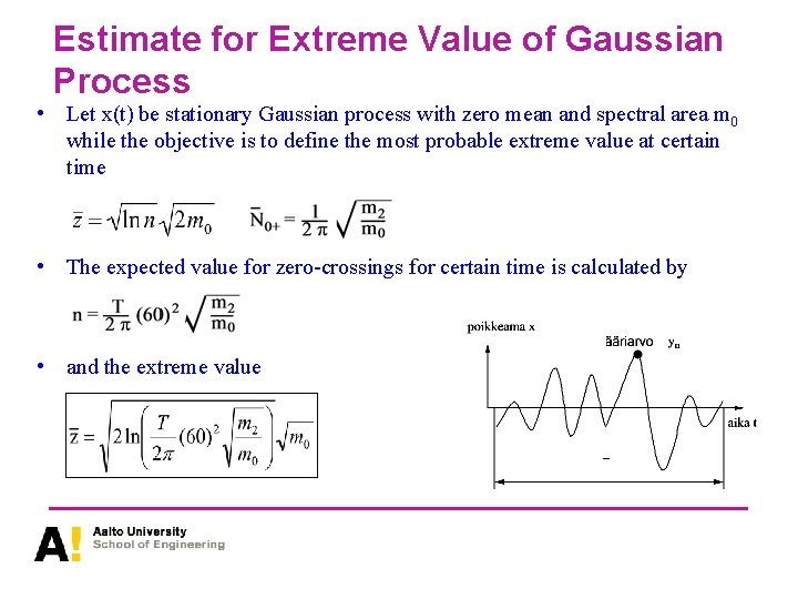
Estimate for Extreme Value of Gaussian Process • Let x(t) be stationary Gaussian process with zero mean and spectral area m 0 while the objective is to define the most probable extreme value at certain time • The expected value for zero-crossings for certain time is calculated by Extreme value • and the extreme value

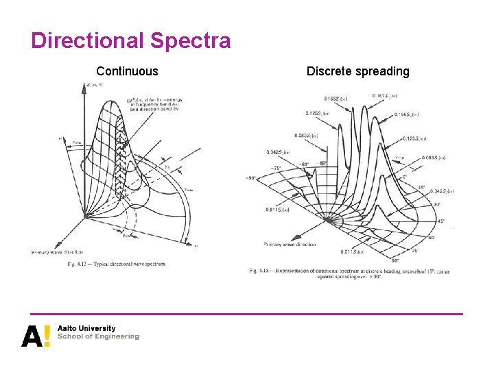
Directional Spectra Continuous Discrete spreading

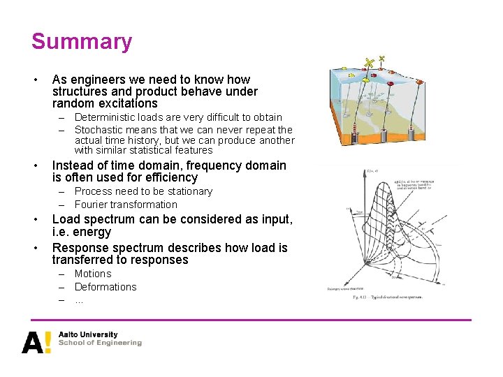
Summary • As engineers we need to know how structures and product behave under random excitations – Deterministic loads are very difficult to obtain – Stochastic means that we can never repeat the actual time history, but we can produce another with similar statistical features • Instead of time domain, frequency domain is often used for efficiency – Process need to be stationary – Fourier transformation • • Load spectrum can be considered as input, i. e. energy Response spectrum describes how load is transferred to responses – Motions – Deformations – …

Aalto University School of Engineering Stochastic Methods in Engineering Probability

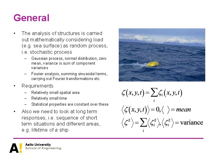
General • • The analysis of structures is carried out mathematically considering load (e. g. sea surface) as random process, i. e. stochastic process – Gaussian process, normal distribution, zero mean, variance is sum of component variances – Fourier analysis, summing sinusoidal terms, carrying out Fourier transformations etc Requirements – – – • Relatively small spatial area Relatively small time Statistical properties are constant over these Also we need to look at long term responses, i. e. sequence of short term situations and different areas, e. g. lifetime of a ship

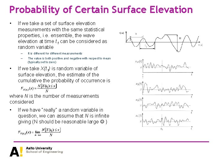
Probability of Certain Surface Elevation • • If we take a set of surface elevation measurements with the same statistical properties, i. e. ensemble, the wave elevation at time t 1 can be considered as random variable – It is different for different measurements – The value is both positive and negative with respect to mean (typically set to zero) If we take X(t 1) is random variable of surface elevation, the estimate of the cumulative the probability of occurrence is where N is the number of measurements considered • If we have “really” a random variable in question, we can assume that N is infinite giving (N should be reasonable large )

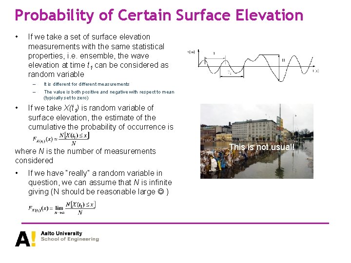
Probability of Certain Surface Elevation • • If we take a set of surface elevation measurements with the same statistical properties, i. e. ensemble, the wave elevation at time t 1 can be considered as random variable – It is different for different measurements – The value is both positive and negative with respect to mean (typically set to zero) If we take X(t 1) is random variable of surface elevation, the estimate of the cumulative the probability of occurrence is where N is the number of measurements considered • If we have “really” a random variable in question, we can assume that N is infinite giving (N should be reasonable large ) This is not usual!

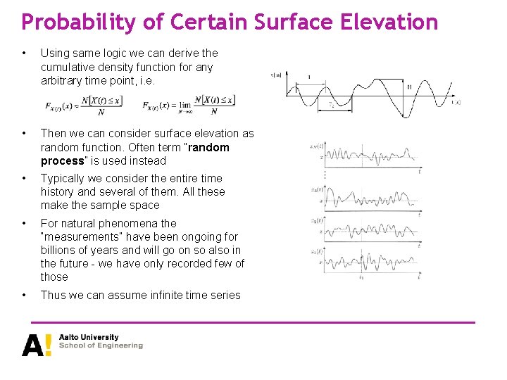
Probability of Certain Surface Elevation • Using same logic we can derive the cumulative density function for any arbitrary time point, i. e. • Then we can consider surface elevation as random function. Often term “random process” is used instead • Typically we consider the entire time history and several of them. All these make the sample space • For natural phenomena the “measurements” have been ongoing for billions of years and will go on so also in the future - we have only recorded few of those • Thus we can assume infinite time series

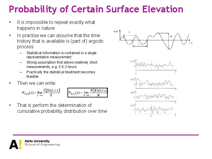
Probability of Certain Surface Elevation • It is impossible to repeat exactly what happens in nature • In practise we can assume that the time history that is available is (part of) ergodic process – Statistical information is contained in a single representative measurement – Strong assumption that allows relatively short measurements, e. g. 0. 5 -3 hours – Practically the statistical treatment becomes feasible • Then we can write • That is perform the determination of cumulative probability distribution over time

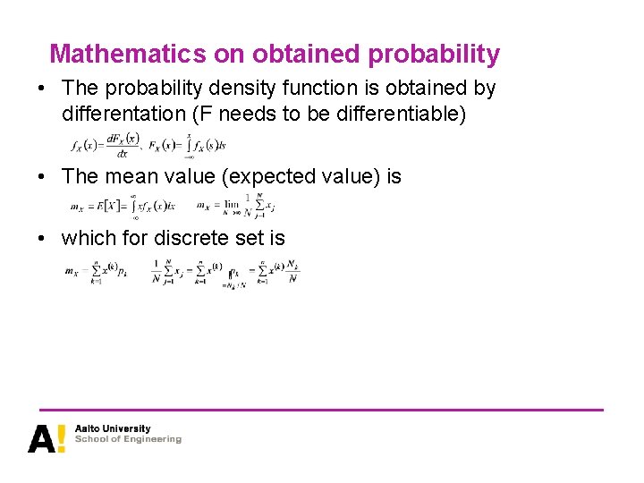
Mathematics on obtained probability • The probability density function is obtained by differentation (F needs to be differentiable) • The mean value (expected value) is • which for discrete set is

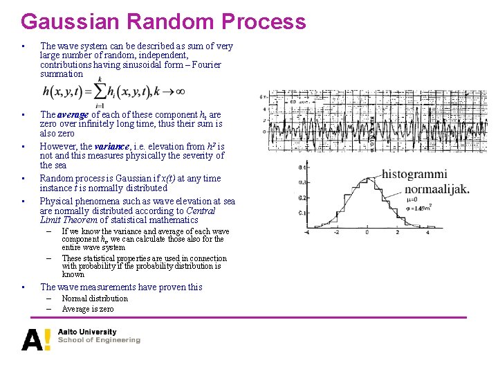
Gaussian Random Process • The wave system can be described as sum of very large number of random, independent, contributions having sinusoidal form – Fourier summation • The average of each of these component hi are zero over infinitely long time, thus their sum is also zero However, the variance, i. e. elevation from h 2 is not and this measures physically the severity of the sea Random process is Gaussian if x(t) at any time instance t is normally distributed Physical phenomena such as wave elevation at sea are normally distributed according to Central Limit Theorem of statistical mathematics • • • – – • If we know the variance and average of each wave component hi, we can calculate those also for the entire wave system These statistical properties are used in connection with probability if the probability distribution is known The wave measurements have proven this – – Normal distribution Average is zero

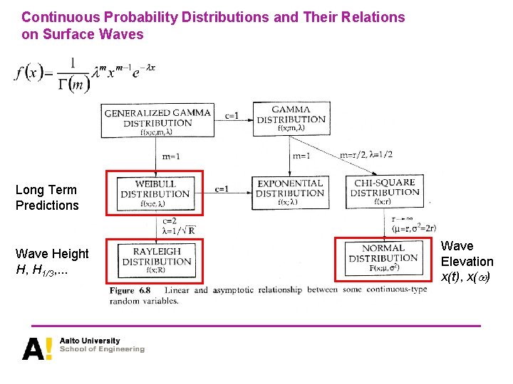
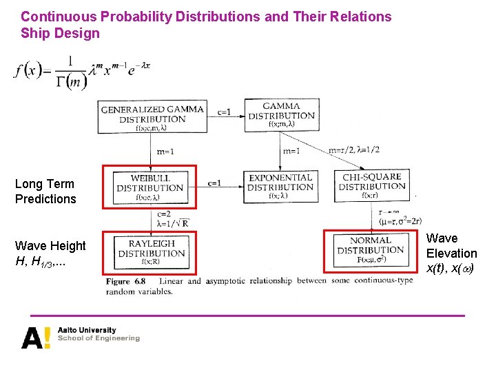
Continuous Probability Distributions and Their Relations on Surface Waves Long Term Predictions Wave Height H, H 1/3, . . . Wave Elevation x(t), x(w)

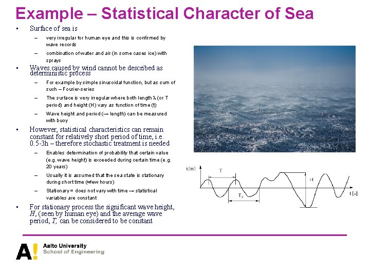
Example – Statistical Character of Sea • • Surface of sea is – very irregular for human eye and this is confirmed by wave records – combination of water and air (in some cases ice) with sprays Waves caused by wind cannot be described as deterministic process – For example by simple sinusoidal function, but as sum of such – Fourier-series – The surface is very irregular where both length l (or T period) and height (H) vary as function of time (t) – Wave height and period (→ length) can be measured with buoy However, statistical characteristics can remain constant for relatively short period of time, i. e. 0. 5 -3 h – therefore stochastic treatment is needed – Enables determination of probability that certain value (e. g. wave height) is exceeded during certain time (e. g. 20 years) – Usually it is assumed that the sea state is stationary during short time ( few hours) – Stationary = does not vary with time → statistical variables are constant For stationary process the significant wave height, H, (seen by human eye) and the average wave period, T, can be considered to be constant

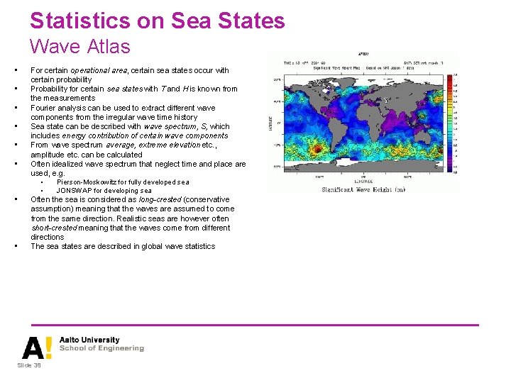
Statistics on Sea States Wave Atlas • • For certain operational area, certain sea states occur with certain probability Probability for certain sea states with T and H is known from the measurements Fourier analysis can be used to extract different wave components from the irregular wave time history Sea state can be described with wave spectrum, S, which includes energy contribution of certain wave components From wave spectrum average, extreme elevation etc. , amplitude etc. can be calculated Often idealized wave spectrum that neglect time and place are used, e. g. • Pierson-Moskowitz for fully developed sea • JONSWAP for developing sea Often the sea is considered as long-crested (conservative assumption) meaning that the waves are assumed to come from the same direction. Realistic seas are however often short-crested meaning that the waves come from different directions The sea states are described in global wave statistics Slide 38

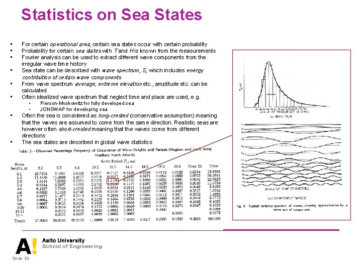
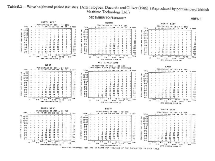
Statistics on Sea States • • For certain operational area, certain sea states occur with certain probability Probability for certain sea states with T and H is known from the measurements Fourier analysis can be used to extract different wave components from the irregular wave time history Sea state can be described with wave spectrum, S, which includes energy contribution of certain wave components From wave spectrum average, extreme elevation etc. , amplitude etc. can be calculated Often idealized wave spectrum that neglect time and place are used, e. g. • Pierson-Moskowitz for fully developed sea • JONSWAP for developing sea Often the sea is considered as long-crested (conservative assumption) meaning that the waves are assumed to come from the same direction. Realistic seas are however often short-crested meaning that the waves come from different directions The sea states are described in global wave statistics Slide 39

Assumed Sea State • North-Atlantic is usually used in design of ship structures – If unlimited operation area is considered – It is not wise to consider this always – too high loads?

Assumed Sea State • North-Atlantic is usually used in design of ship structures – If unlimited operation area is considered – It is not wise to consider this always – too high loads?

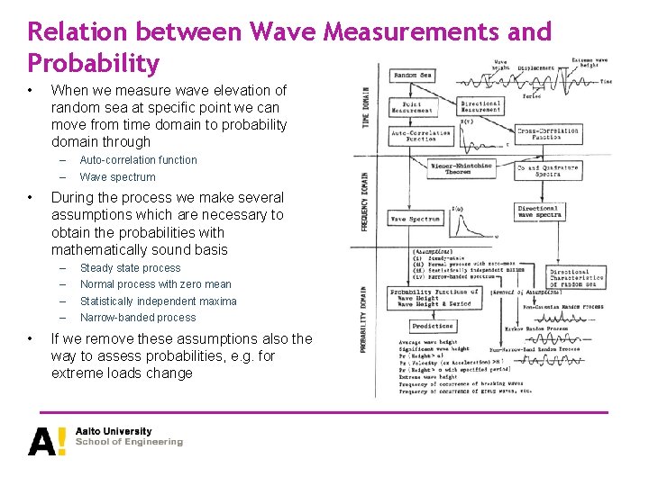
Relation between Wave Measurements and Probability • When we measure wave elevation of random sea at specific point we can move from time domain to probability domain through – – • Wave spectrum During the process we make several assumptions which are necessary to obtain the probabilities with mathematically sound basis – – • Auto-correlation function Steady state process Normal process with zero mean Statistically independent maxima Narrow-banded process If we remove these assumptions also the way to assess probabilities, e. g. for extreme loads change

Parameters/Characteristics of Response Spectrum The kth moment (analogous to mechanics) Narrow band The average angular velocity The kth moment with respect to average angular velocity The bandwith parameter (0 for narrow band 1 for broad band) Broad band

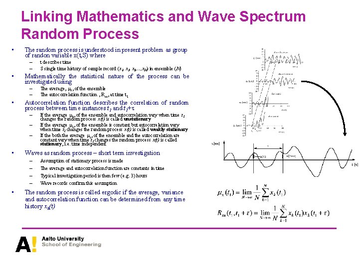
Linking Mathematics and Wave Spectrum Random Process • The random process is understood in present problem as group of randon variable x(t, S) where – – • Mathematically the statistical nature of the process can be investigated using – – • – – If the average x, of the ensemble and autocorrelation vary when time t 1 changes the random process x(t) is called unstationary If the average x, of the ensemble is constant but autocorrelation vary when time t 1 changes the random process x(t) is called weakly stationary If the both the average x, of the ensemble and the autocorrelation are constant vary when time t 1 changes the random process x(t) is called stationary, i. e. time independent Waves as random process – short term investigation – – • The average, x, of the ensemble The autocorrelation function , Rxx, at time t 1 Autocorrelation function describes the correlation of random process between time instances t 1 and t 1+t – • t describes time S single time history of sample record (x 1, x 2, x 3, . . . , x. N) in ensemble (N) Assumption of stationary process is made The average and autocorrelation function are constants in time Typical investigation period is then few (e. g. 3) hours Wave records confirm this assumption The random process is called ergodic if the average, variance and autocorrelation function can be determined from any time history xk(t)

Estimate for Extreme Value of Gaussian Process • Let x(t) be stationary Gaussian process with zero mean and spectral area m 0 while the objective is to define the most probable extreme value at certain time • The expected value for zero-crossings for certain time is calculated by • and the extreme value

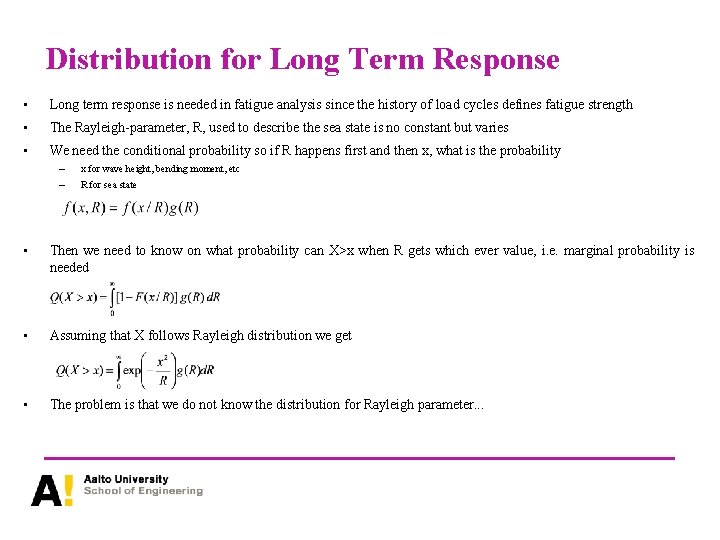
Distribution for Long Term Response • Long term response is needed in fatigue analysis since the history of load cycles defines fatigue strength • The Rayleigh-parameter, R, used to describe the sea state is no constant but varies • We need the conditional probability so if R happens first and then x, what is the probability – x for wave height, bending moment, etc – R for sea state • Then we need to know on what probability can X>x when R gets which ever value, i. e. marginal probability is needed • Assuming that X follows Rayleigh distribution we get • The problem is that we do not know the distribution for Rayleigh parameter. . .

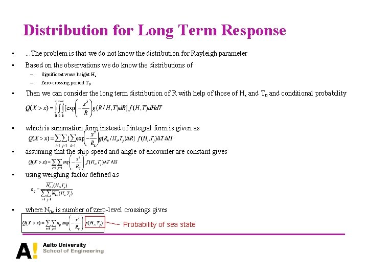
Distribution for Long Term Response • . . . The problem is that we do not know the distribution for Rayleigh parameter • Based on the observations we do know the distributions of – Significant wave height Hs – Zero-crossing period T 0 • Then we can consider the long term distribution of R with help of those of Hs and T 0 and conditional probability • which is summation form instead of integral form is given as • assuming that the ship speed angle of encounter are constant gives • using weighing factor defined as • where N 0 s is number of zero-level crossings gives Probability of sea state

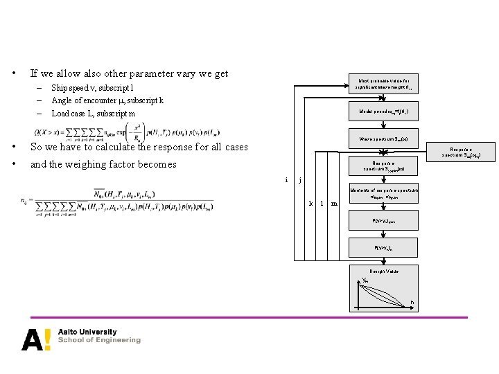
• If we allow also other parameter vary we get – – – Most probable value for significant wave height Hsi Ship speed v, subscript l Angle of encounter , subscript k Modal period wmj=fj(Hs) Load case L, subscript m • So we have to calculate the response for all cases • and the weighing factor becomes Wave spectrum Sxx(w) Response spectrum Sxxj(wmj) Response spectrum Syyijklm(w) i j k l m Moments of response spectrum m 0 ijklm, m 2 jjklm P(y>yw)ijklm P(y>yw)w Design Value yw n

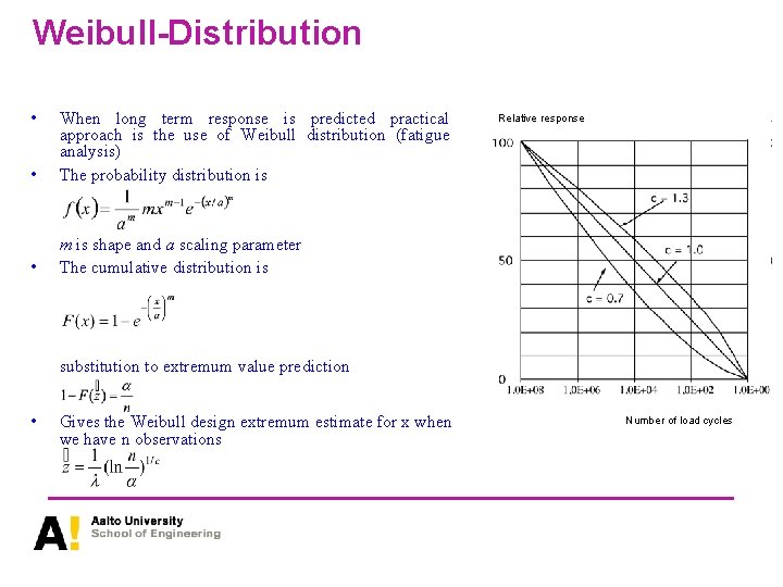
Weibull-Distribution • • When long term response is predicted practical approach is the use of Weibull distribution (fatigue analysis) The probability distribution is • m is shape and a scaling parameter The cumulative distribution is Relative response substitution to extremum value prediction • Gives the Weibull design extremum estimate for x when we have n observations Number of load cycles

Continuous Probability Distributions and Their Relations Ship Design Long Term Predictions Wave Height H, H 1/3, . . . Wave Elevation x(t), x(w)

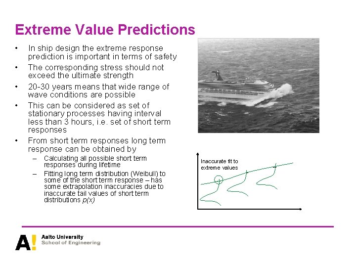
Extreme Value Predictions • • • In ship design the extreme response prediction is important in terms of safety The corresponding stress should not exceed the ultimate strength 20 -30 years means that wide range of wave conditions are possible This can be considered as set of stationary processes having interval less than 3 hours, i. e. set of short term responses From short term responses long term response can be obtained by – Calculating all possible short term responses during lifetime – Fitting long term distribution (Weibull) to some of the short term response – has some extrapolation inaccuracies due to inaccurate tail values of short term distributions p(x) Inaccurate fit to extreme values

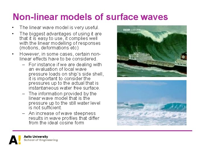
Non-linear models of surface waves • • • The linear wave model is very useful. The biggest advantages of using it are that it is easy to use, it complies well with the linear modelling of responses (motions, deformations etc) However, in some cases, certain nonlinear effects have to be considered. – For instance if we are dealing with an evaluation of local wave pressure loads on ship’s side shell, it is important to consider the pressures up to the actual that is instantaneous water free surface. – The information provided by the linear wave model that is the pressure up to the still water level is not sufficient. – An increase of wave steepness results in wave profiles that differ from the ideal cosine form

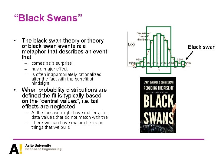
“Black Swans” • The black swan theory or theory of black swan events is a metaphor that describes an event that – comes as a surprise, – has a major effect – is often inappropriately rationalized after the fact with the benefit of hindsight • When probability distributions are defined the fit is typically based on the “central values”, i. e. tail effects are neglected – At the tails we might have outliers, i. e. data values that do not match with the – There we can have major effects on things that we build Black swan

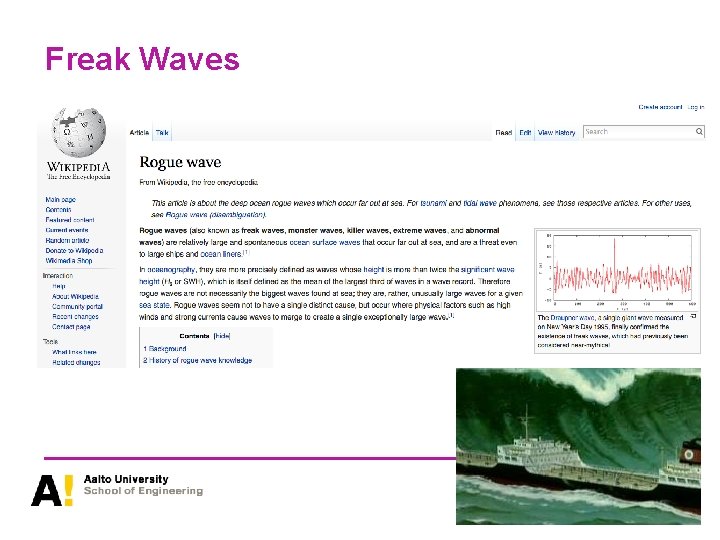
Freak Waves

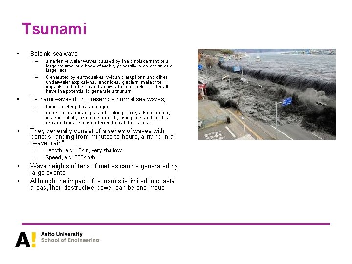
Tsunami • Seismic sea wave – – • Tsunami waves do not resemble normal sea waves, – – • • their wavelength is far longer rather than appearing as a breaking wave, a tsunami may instead initially resemble a rapidly rising tide, and for this reason they are often referred to as tidal waves. They generally consist of a series of waves with periods ranging from minutes to hours, arriving in a "wave train” – – • a series of water waves caused by the displacement of a large volume of a body of water, generally in an ocean or a large lake Generated by earthquakes, volcanic eruptions and other underwater explosions, landslides, glaciers, meteorite impacts and other disturbances above or below water all have the potential to generate a tsunami Length, e. g. 10 km, very shallow Speed, e. g. 800 km/h Wave heights of tens of metres can be generated by large events Although the impact of tsunamis is limited to coastal areas, their destructive power can be enormous

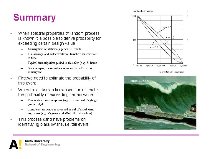
Summary • When spectral properties of random process is known it is possible to derive probability for exceeding certain design value – – Assumption of stationary process is made – – Typical investigation period is then few (e. g. 3) hours The average and autocorrelation function are constants in time For example, measured wave records confirm this assumption • First we need to estimate the probability of this event • When this is known we can estimate the probability of exceeding certain value • – This is short term response (e. g. 3 hours and Rayleight probability) – Long term response is assessed as set of short term responses (e. g. 25 years and Weibull distribution) This process cand have problems on identifuying black swans, i. e. tail event