7 4 Nyquist Stability Criterion 1 Introduction to

7 -4 Nyquist Stability Criterion

1. Introduction to Nyquist stability criterion The Nyquist stability criterion determines the stability of a closed-loop system from its open-loop frequency response and open-loop poles, and there is no need for actually determining the closed-loop poles. To determine the stability of a closed-loop system, one must investigate the closed-loop characteristic equation of the system.

We consider the following typical closed-loop system: where From the above diagram, we have We define

which is also called the characteristic equation of the closed-loop system and will play an important role in stability analysis. In fact, we have Further, we assume that deg(N 1 N 2)<deg(D 1 D 2), which implies that both the denominator and nominator polynomials of F(s) have the same degree.

2. Preliminary Study Consider, for example, the following open-loop transfer function: whose closed-loop characteristic equation is which is analytic everywhere except at its singular points. For each point analytic in s plane, F(s) maps the point into F(s) plane. For example, s=2+j: F(s)=2 j. Further, we have the following conclusion:

Conformal mapping: For any given continuous closed path in the s plane that does not go through any singular points, there corresponds a closed curve in the F(s) plane. s-plane F(s) plane

Example. Consider Case 1: s-plane F(s)-Plane A B -1 1 0 G G ׳ D H -2 C 2 F s: clockwise 3 E -1 0 E ׳ D ׳ H ׳ 1 C ׳ 2 3 A ׳ F: clockwise F encircles the origin:

Case 2: F(s) plane s-plane A B E ׳ D H -2 G C F 1 E s: clockwise 0 D ׳ -1 G ׳ 0 A ׳ 1 C ׳ F: clockwise F encircles the origin:

Case 3: F ׳ s-plane A B C D H -2 G F E s: clockwise E ׳ G ׳ H ׳ D ׳ -1 0 -1 F(s) plane 0 1 C ׳ A ׳ B ׳ F: counterclockwise F encircles the origin:

Case 4: It can be verified that when s encloses both the pole and zero in the clockwise direction, the number of the F encircles the origin is 1+1=0.

If, for example, F(s) has two zeros and one pole are enclosed by s, it can be deduced from the above analysis that F encircles the origin of F plane one time in the clockwise direction as s traces out s.

Mapping theorem (The principle of argument) Let F(s) be a ratio of two polynomials in s. Let P be the number of poles and Z be the number of zeros of F(s) that lie inside a closed contour s, which does not pass through any poles and zeros of F(s). Then the s in the s-plane is mapped into the F(s) plane as a closed curve, F. The total number N of counterclockwise encirclements of the origin of the F(s), as s traces out s in the clockwise direction, is equal to N=P Z

3. The Nyquist Stability Criterion For a stable system, all the zeros of F(s) must lie in the left-half s-plane.

Therefore, we choose a contour s, say, Nyquist path, in the s-plane that encloses the entire right-half s-plane. The contour consists of the entire j axis ( varies from to + ) and a semicircular path of infinite radius in the right-half s plane. Nyquist contour As a result, the Nyquist path encloses all the zeros and poles of F(s)=1+G(s)H(s) that have positive real parts. s-plane

Now, let P be the number of the unstable open-loop poles, which is assumed to be known, N be the number of encirclements of the origin of F(s) in counterclockwise direction, which, by drawing the curve, is also known, and Z be the number of the unstable closed-loop poles, which is unknown. Then by applying the Mapping Theorem, we have N=P Z. If Z=0, the system is stable; if Z>0, the system is unstable with the number of unstable poles being Z. Question: How to obtain the curve of F(s) as s traces out s in clockwise direction?

By assumption, Nyquist contour s-plane It is clear that when s traverses the semicircle of infinite radius, F(s) remains a constant. That is, the encirclements of the origin of F(s) only determines by F(j ) as varies from to + provided that no zeros or poles lie on the j axis.

Example. Consider a unity feedback system whose open-loop transfer function is as follows F(j ) The system is stable.

Further, since compare the two curves below: F(j ) GH(j ) Clearly, the encirclement of the origin in F plane is equivalent to the encirclement of 1 point in GH plane!

Example. Consider a unity feedback system whose open-loop transfer function is as follows G(s) The system is unstable.

Example. Consider a single-loop control system, where Determine its stability. The system is stable. G(s)H(s)

Nyquist stability criterion A system is stable if and only if from N = P Z we can obtain that Z=0, where P is the number of the open -loop poles in the right-hand half s-plane and N is the number of the encirclements of the point ( 1, j 0) of G(j )H(j ) in the counterclockwise direction.

Because the plot of G(j )H(j ) and the plot of G( j )H( j ) are symmetrical with each other about the real axis. Hence, we can modify the stability criterion as N = (P – Z)/2, where only the polar plot of G(j )H(j ) with varying from 0 to + is necessary. Im Im Re -1 0 Re -1 G(s)H(s) 0 G(s)H(s)

Example. Consider a unity feedback system whose open-loop transfer function is as follows Investigate its stability by using Nyquist criterion. Solution: Obviously, P=1 (nonminimum phase plant). Now, drawing its Nyquist plot yields: G(j ) The system is stable.

Example. Consider a unity feedback system whose open-loop transfer function is as follows Using Nyquist plot, determine its stability. Solution: Obviously, P=0. Now, drawing its Nyquist plot yields:

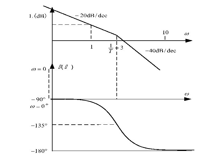
4. Nyquist Criterion Based on Bode diagram Again, we consider the open-loop transfer function with Nyquist curve below: where P=0, N= 1 and the system is unstable. The key is the point that the Nyquist curve crosses the negative real axis is less than 1 (abs(A)>1).

The Bode diagram is: N =1 The system is unstable because the phase angle plot crosses the 1800 line in the region of 20 log G(j ) >0.

We use N to denote the number of crosses of 1800 line in the region of 20 log G(j ) >0 if each across makes the phase angle less than 1800. Similarly, we use N+ to denote the number of crosses of 1800 line in the region of 20 log G(j ) >0 if each across makes the phase angle larger than 1800. The Nyquist Theorem can be interpreted as: Theorem: The system is stable if and only if from N+ N = (P – Z)/2 we can obtain that Z=0.

Example. Both the Nyquist plot and Bode diagram of an open-loop minimum phase transfer function are shown below. Determine its stability.

5. Special case when G(s)H(s) involves Poles and Zeros on the j Axis Consider the following open-loop transfer function: which does not satisfy the Nyquist Theorem because s is a singular point. Therefore, the contour s must be modified. A way of modifying the contour near the origin is to use a quarter-circle with an infini-tesimal radius (>0): where varies from 00 to 900 as varies from 0 to 0+.

A modified contour s : The modified s implies that we regard 1/s as a stable pole. s-plane j 0+ =0 Then, for the controlled plant with integral factor 1/s, we have where 1/s rotates from 00 to 900 with an infinite radius as varies from 0 to 0+.

j =0 j 0+ The integral factor 1/s rotates from 00 to 900 with an infinite radius as varies from 0 to 0+.

s-plane GH-plane C B’ B -1 C’ The Nyquist curve starts from real axis when =0 and rotates 900 as =0+. N = (P – Z)/2 Z=0, the system is stable.

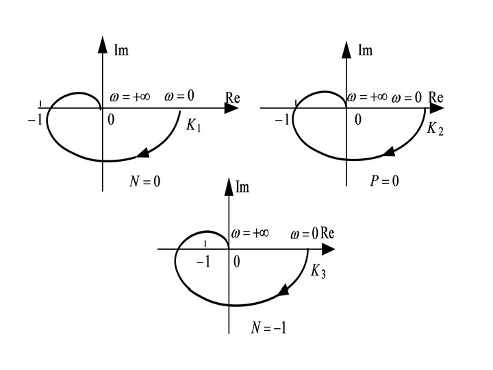
Example. Let the open-loop transfer function be Determine its stability by using Nyquist Theorem. Solution: When =0, When =0+, Hence, when >0+,

P=0, N= 1 N=(P Z)/2 Z=2. The system is unstable.

P=0, N =1, N+=0 N+ N =(P Z)/2 Z=2. The system is unstable.

6. Stability Analysis Example. Let the open-loop transfer function be Determine its stability by using Nyquist Theorem. Solution: When =0, When =0+ Hence, when >0+,

If T 1>T 2, the Nyquist curve is shown below. Since P=0, N= 1 N=(P Z)/2 Z=2. The system is unstable.

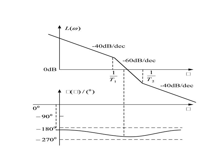
If T 2>T 1, the Nyquist curve is shown below. Since P=0, N=0 N=(P Z)/2 Z=0. The system is stable.

P=0, N =1/2, N+=1/2 N+ N =(P Z)/2 Z=0. The system is stable.

Example. Consider a unity feedback system whose open-loop transfer function is as follows Investigate its stability by using Nyquist criterion. Solution: Obviously, P=1 (nonminimum phase plant). Now, drawing its Nyquist plot yields: The system is unstable.

7. Conditionally Stable Systems A conditionally stable system is stable for the value of the open-loop gain lying between critical values, but it is unstable if the open-loop gain is either increased or decreased sufficiently.

Example. Consider a single-loop control system, where open-loop transfer function is Determine the range of K so that the system keeps stable.

Example. Consider a single-loop control system, where open-loop transfer function is Discuss its stability by using Nyquist stability criterion.