Bode Plot Bode Plot for Gssa Let sj

Bode Plot
=s+a • Let s=jω, G(jω)=jω+a= • At low frequencies, when ω")
Bode Plot for G(s)=s+a • Let s=jω, G(jω)=jω+a= • At low frequencies, when ω approach zero, G(jω)≈a The magnitude response in d. B is 20 log M=20 log a, where , a constant from ω=0. 01 a to a. • At high frequencies, ω>>a, G(jω)≈ The magnitude response in d. B is 20 log M=20 log a + 20 log =20 log ω, where , y=20 x, straight line

• We call the low frequency approximation and high frequency approximation with the term low frequency asymptote and high frequency asymptote respectively. • The frequency, a, is called the break frequency. • As for phase response, at low frequency , the phase=0 o, at high frequency, phase=90 o. • To draw the curve, start one decade (1/10) below the break frequency (0. 1 a) , draw a line of slope +45 o/decade passing through 45 o at the break frequency and continue to 90 o at one decade above the break frequency (10 a).

![• To normalize (s+a), we factor out a and form a[(s/a)+1]. • By](http://slidetodoc.com/presentation_image_h/cfa262d05fbe90ba22784c0623460941/image-5.jpg "• To normalize (s+a), we factor out a and form a[(s/a)+1]. • By")
• To normalize (s+a), we factor out a and form a[(s/a)+1]. • By defining a new frequency variable, s 1=s/a, then the magnitude is divided by a to yield 0 d. B at the break frequency. • The normalized and scaled function is (s 1+1). • To obtain the original frequency response, the magnitude and frequency is multiplied by a.

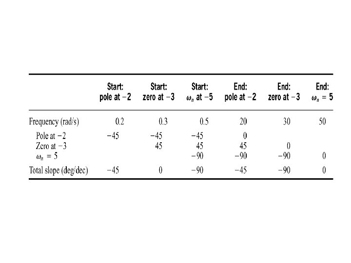
Table 10. 1 Asymptotic and actual normalized and scaled frequency response data for (s + a)

Figure 10. 7 Asymptotic and actual normalized and scaled magnitude response of (s + a)

Figure 10. 8 Asymptotic and actual normalized and scaled phase response of (s + a)
=1/(s+a) The function has a low frequency asymptote of 20 log(1/a),")
Bode Plot for G(s)=1/(s+a) The function has a low frequency asymptote of 20 log(1/a), when s approach zero. The Bode plot is constant until break frequency, a rad/s is reached. At high frequency asymptote, when s approach infinity,
 = s; b. G(s) = 1/s;")
Normalized and scaled Bode plots for a. G(s) = s; b. G(s) = 1/s; c. G(s) = (s + a); d. G(s) = 1/(s + a)
![Draw the Bode Plots for the system shown below, G(s)=K(s+3)/[s(s+1)(s+2)] The break frequencies are](http://slidetodoc.com/presentation_image_h/cfa262d05fbe90ba22784c0623460941/image-11.jpg "Draw the Bode Plots for the system shown below, G(s)=K(s+3)/[s(s+1)(s+2)] The break frequencies are")
Draw the Bode Plots for the system shown below, G(s)=K(s+3)/[s(s+1)(s+2)] The break frequencies are at 1, 2, 3. The magnitude plot should begin a decade below the lowest break frequency and extend to a decade above the highest break frequency. Hence, we choose 0. 1 rad to 100 rad for this plot. The effect of K is to move the magnitude curve up and down by the amount of 20 log K. K has no effect on the phase curve. Let K=1 in this case.

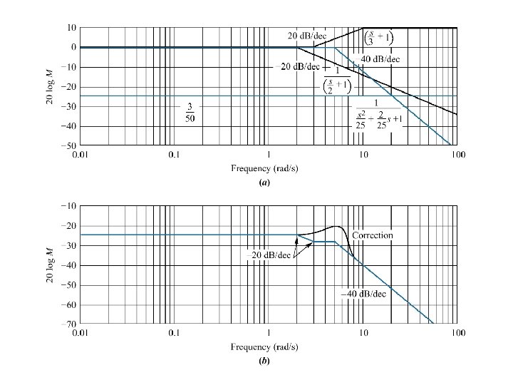
Magnitude Plot:

Bode log-magnitude plot: a. components; b. composite

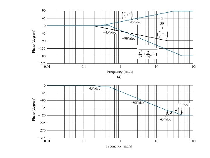
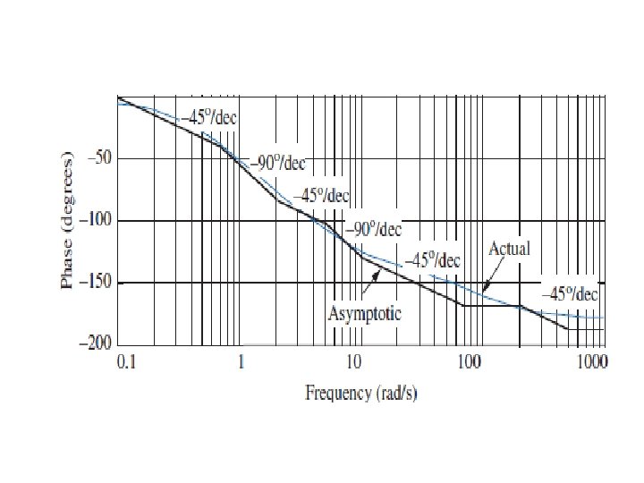
Phase Plot:
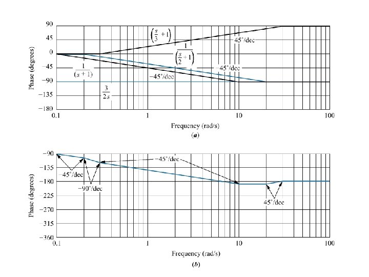

Bode Plot for The straight line is twice the slope of a first order term which is 40 d. B/decade.
 = a. magnitude; b. phase")
Bode asymptotes for normalized and scaled G(s) = a. magnitude; b. phase

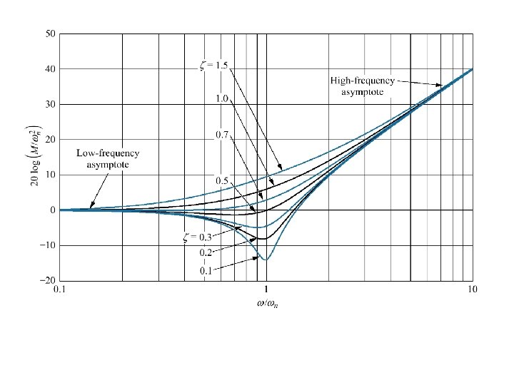
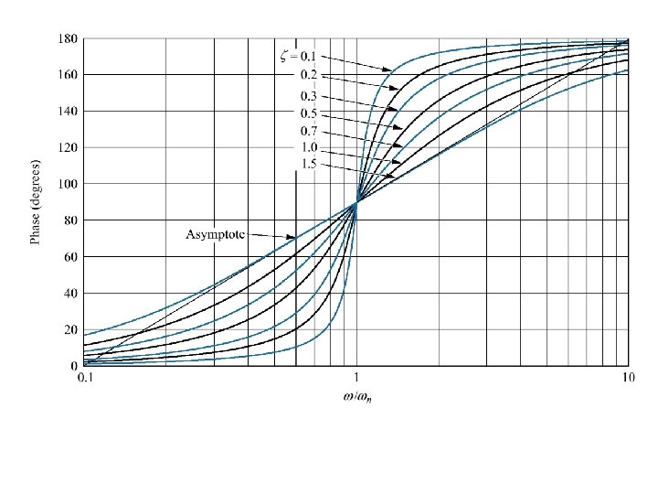
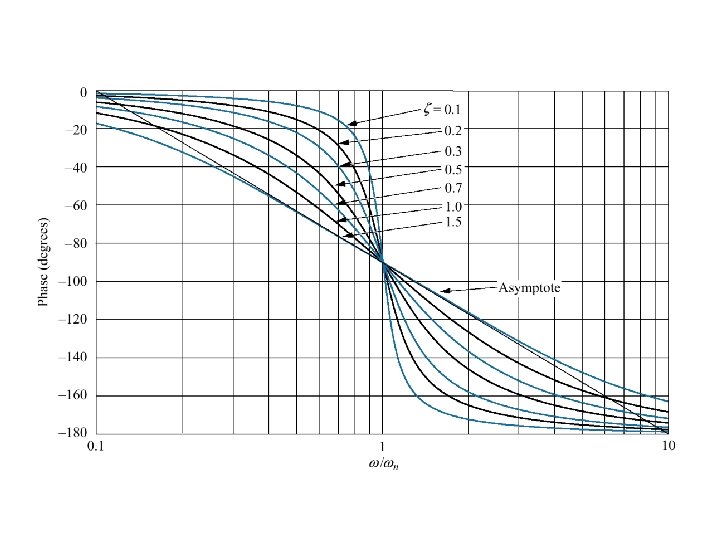
• In second order polynomial, ωn is the break frequency. • For normalization, we divide the magnitude by ωn 2, and scale the frequency , dividing by ωn. Thus, • G(s 1) has a low frequency asymptote at 0 d. B and a break frequency of 1 rad/s. • For the phase plot, it is at 0 o at low frequencies and 180 o at high frequencies. The phase plot increase at a rate of 90 o/decade from 0. 1 to 10 and passes through 90 o at 1. • The error between the actual response and the asymptotic approximation of the second order polynomial can be great depending on the value of ζ. • The actual magnitude and phase for are:

Bode Plot for
 for an unity feedback system.")
Draw the Bode log-magnitude and phase plots of G(s) for an unity feedback system.

Exercise: • Draw the Bode log-magnitude and phase plots for the system below:

Answer:

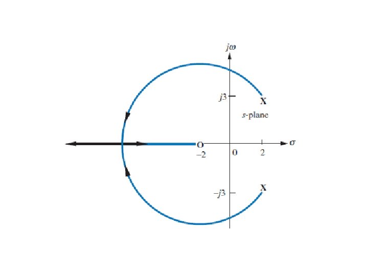
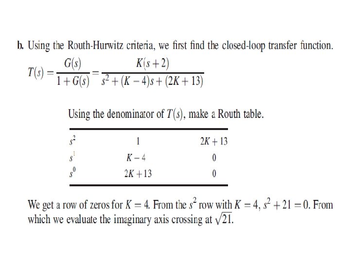
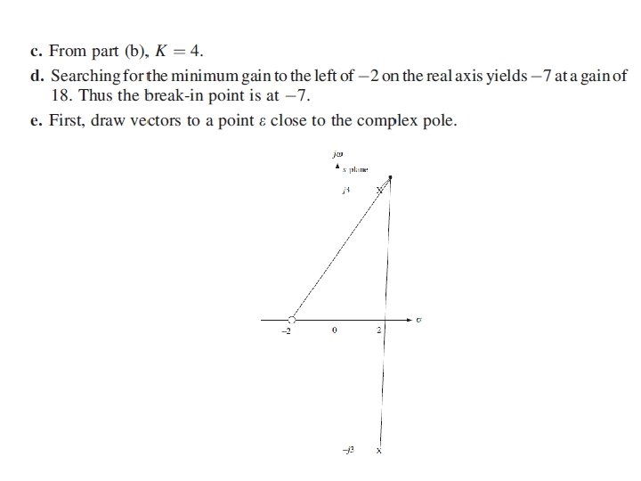
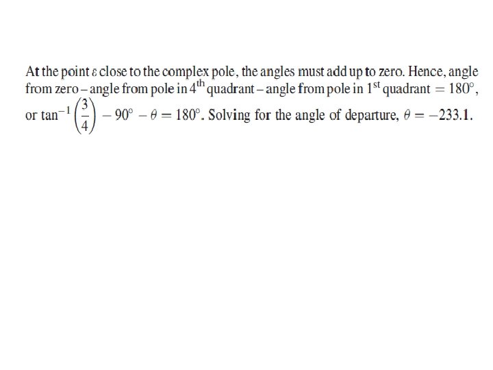
Exercise: Root Locus • Given a unity feedback system with the forward transfer function: • • • Sketch the root locus Find the imaginary-axis crossing Find Gain K at jω-axis crossing Find the break-in point Find the angle of departure from the upper plane complex pole
- Slides: 34