Lecture 22 Kelly Criterion and Utility John Rundle

Lecture 22 Kelly Criterion and Utility John Rundle Econophysics PHYS 250

Kelly Criterion https: //en. wikipedia. org/wiki/Kelly_criterion • In probability theory and intertemporal portfolio choice, the Kelly criterion, Kelly strategy, Kelly formula, or Kelly bet, is a formula used to determine the optimal size of a series of bets. • In most gambling scenarios, and some investing scenarios under some simplifying assumptions, the Kelly strategy will do better than any essentially different strategy in the long run (that is, over a span of time in which the observed fraction of bets that are successful equals the probability that any given bet will be successful). • It was described by J. L. Kelly, Jr, a researcher at Bell Labs, in 1956. • In recent years, Kelly has become a part of mainstream investment theory[8] and the claim has been made that well-known successful investors including Warren Buffett[9] and Bill Gross[10] use Kelly methods. William Poundstone wrote an extensive popular account of the history of Kelly betting. [6]

Kelly Criterion https: //en. wikipedia. org/wiki/Kelly_criterion • The Kelly Criterion is to bet a predetermined fraction of assets and can be counterintuitive. • In one study, each participant was given $25 and asked to bet on a coin that would land heads 60% of the time. • The prizes were capped at $250. "Remarkably, 28% of the participants went bust, and the average payout was just $91. • Only 21% of the participants reached the maximum. 18 of the 61 participants bet everything on one toss, while two-thirds gambled on tails at some stage in the experiment. • Neither approach is in the least bit optimal. " • Using the Kelly criterion and based on the odds in the experiment, the right approach would be to bet 20% of the pot on each throw (see first example in Statement below). • If losing, the size of the bet gets cut; if winning, the stake increases.

Kelly Criterion https: //en. wikipedia. org/wiki/Kelly_criterion • Although the Kelly strategy's promise of doing better than any other strategy in the long run seems compelling, some economists have argued strenuously against it, mainly because an individual's specific investing constraints may override the desire for optimal growth rate. • The conventional alternative is expected utility theory which says bets should be sized to maximize the expected utility of the outcome (to an individual with logarithmic utility, the Kelly bet maximizes expected utility, so there is no conflict • Moreover, Kelly's original paper clearly states the need for a utility function in the case of gambling games which are played finitely many times). • Even Kelly supporters usually argue for fractional Kelly (betting a fixed fraction of the amount recommended by Kelly) for a variety of practical reasons, such as wishing to reduce volatility, or protecting against nondeterministic errors in their advantage (edge) calculations.

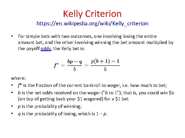
Kelly Criterion https: //en. wikipedia. org/wiki/Kelly_criterion • For simple bets with two outcomes, one involving losing the entire amount bet, and the other involving winning the bet amount multiplied by the payoff odds, the Kelly bet is: where: • f* is the fraction of the current bankroll to wager, i. e. how much to bet; • b is the net odds received on the wager ("b to 1"); that is, you could win $b (on top of getting back your $1 wagered) for a $1 bet • p is the probability of winning; • q is the probability of losing, which is 1 − p.

Kelly Criterion https: //en. wikipedia. org/wiki/Kelly_criterion • As an example, if a gamble has a 60% chance of winning (p = 0. 60, q = 0. 40), and the gambler receives 1 -to-1 odds on a winning bet (b = 1), then the gambler should bet 20% of his bankroll at each opportunity (f* = 0. 20), in order to maximize the long-run growth rate of the bankroll. • If the gambler has zero edge, i. e. if b = q / p, then the criterion recommends the gambler bets nothing. • If the edge is negative (b < q / p) the formula gives a negative result, indicating that the gambler should take the other side of the bet.

Kelly Criterion https: //en. wikipedia. org/wiki/Kelly_criterion • For example, in standard American roulette, the bettor is offered an even money payoff (b = 1) on red, when there are 18 red numbers and 20 non-red numbers on the wheel (p = 18/38). • The Kelly bet is -1/19, meaning the gambler should bet onenineteenth of his bankroll that red will not come up. • Unfortunately, the casino doesn't allow betting against something coming up, so a Kelly gambler cannot place a bet.

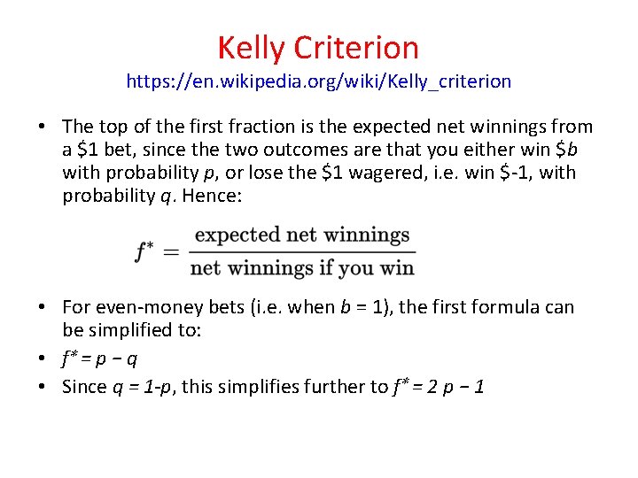
Kelly Criterion https: //en. wikipedia. org/wiki/Kelly_criterion • The top of the first fraction is the expected net winnings from a $1 bet, since the two outcomes are that you either win $b with probability p, or lose the $1 wagered, i. e. win $-1, with probability q. Hence: • For even-money bets (i. e. when b = 1), the first formula can be simplified to: • f∗ = p − q • Since q = 1 -p, this simplifies further to f∗ = 2 p − 1

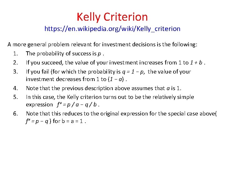
Kelly Criterion https: //en. wikipedia. org/wiki/Kelly_criterion A more general problem relevant for investment decisions is the following: 1. The probability of success is p. 2. If you succeed, the value of your investment increases from 1 to 1 + b. 3. If you fail (for which the probability is q = 1 − p, the value of your investment decreases from 1 to (1 − a). 4. Note that the previous description above assumes that a is 1. 5. In this case, the Kelly criterion turns out to be the relatively simple expression f∗ = p / a − q / b. 6. Note that this reduces to the original expression for the special case above( f∗ = p − q ) for b = a = 1.

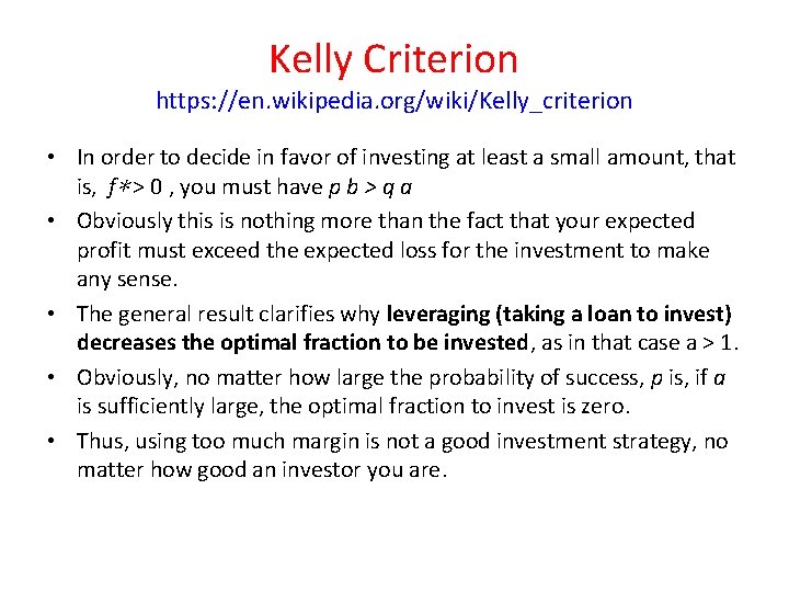
Kelly Criterion https: //en. wikipedia. org/wiki/Kelly_criterion • In order to decide in favor of investing at least a small amount, that is, f∗ > 0 , you must have p b > q a • Obviously this is nothing more than the fact that your expected profit must exceed the expected loss for the investment to make any sense. • The general result clarifies why leveraging (taking a loan to invest) decreases the optimal fraction to be invested, as in that case a > 1. • Obviously, no matter how large the probability of success, p is, if a is sufficiently large, the optimal fraction to invest is zero. • Thus, using too much margin is not a good investment strategy, no matter how good an investor you are.

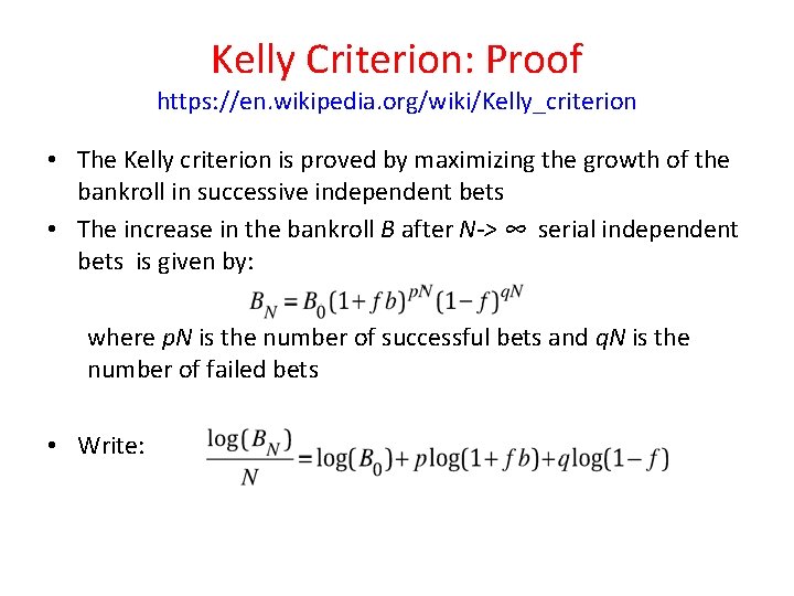
Kelly Criterion: Proof https: //en. wikipedia. org/wiki/Kelly_criterion • The Kelly criterion is proved by maximizing the growth of the bankroll in successive independent bets • The increase in the bankroll B after N-> ∞ serial independent bets is given by: where p. N is the number of successful bets and q. N is the number of failed bets • Write:

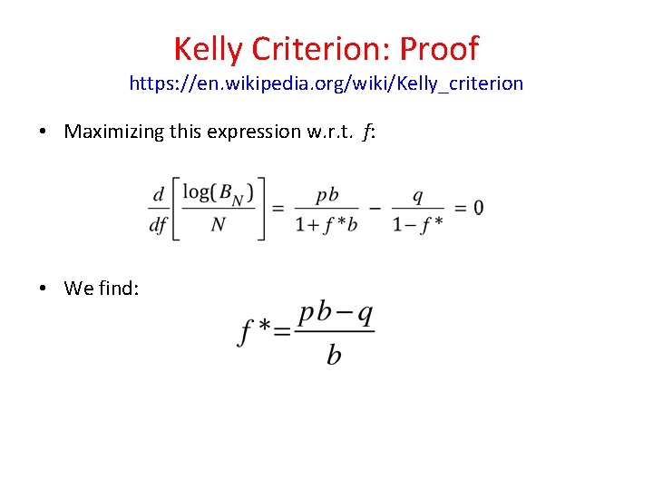
Kelly Criterion: Proof https: //en. wikipedia. org/wiki/Kelly_criterion • Maximizing this expression w. r. t. f: • We find:

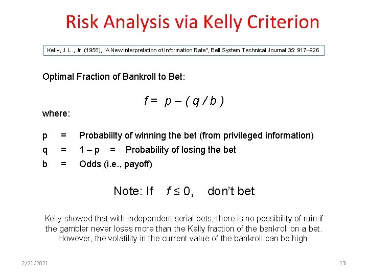
Risk Analysis via Kelly Criterion Kelly, J. L. , Jr. (1956), "A New Interpretation of Information Rate", Bell System Technical Journal 35: 917– 926 Optimal Fraction of Bankroll to Bet: f= p–(q/b) where: p = Probabiilty of winning the bet (from privileged information) q = 1–p b = Odds (i. e. , payoff) = Probability of losing the bet Note: If f ≤ 0, don’t bet Kelly showed that with independent serial bets, there is no possibility of ruin if the gambler never loses more than the Kelly fraction of the bankroll on a bet. However, the volatility in the current value of the bankroll can be high. 2/21/2021 13

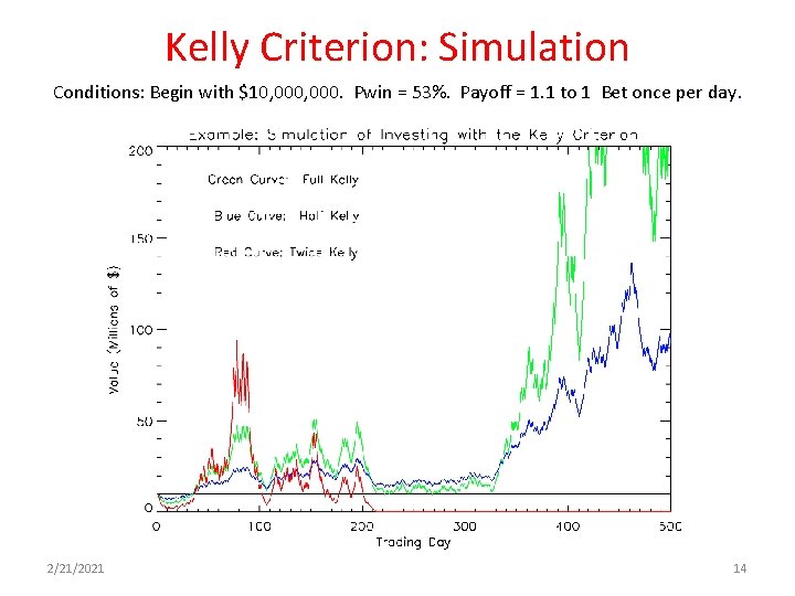
Kelly Criterion: Simulation Conditions: Begin with $10, 000. Pwin = 53%. Payoff = 1. 1 to 1 Bet once per day. 2/21/2021 14

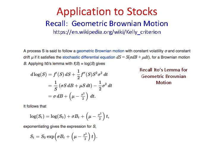
Application to Stocks Recall: Geometric Brownian Motion https: //en. wikipedia. org/wiki/Kelly_criterion Recall Ito’s Lemma for Geometric Brownian Motion

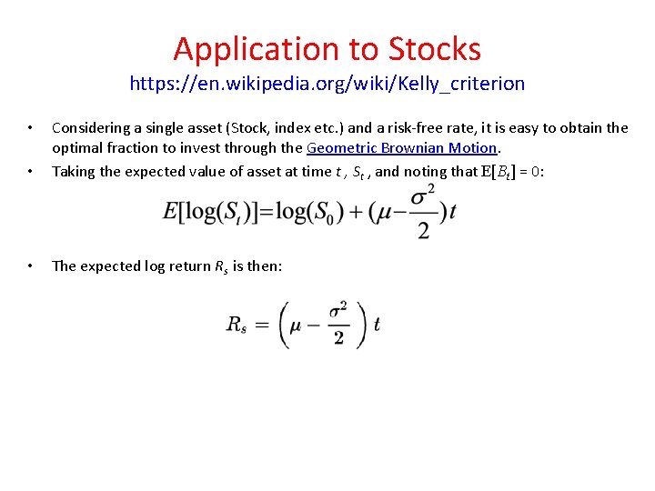
Application to Stocks https: //en. wikipedia. org/wiki/Kelly_criterion • Considering a single asset (Stock, index etc. ) and a risk-free rate, it is easy to obtain the optimal fraction to invest through the Geometric Brownian Motion. Taking the expected value of asset at time t , St , and noting that E[Bt] = 0: • The expected log return Rs is then: •

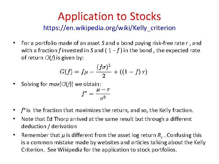
Application to Stocks https: //en. wikipedia. org/wiki/Kelly_criterion • For a portfolio made of an asset S and a bond paying risk-free rate r , and with a fraction f invested in S and ( 1 − f ) in the bond , the expected rate of return G(f) is given by: • Solving for max[G(f)] we obtain: • f∗ is the fraction that maximizes the return, and so, the Kelly fraction. • Note that Ed Thorp arrived at the same result but through a different deduction / derivation • Remember that μ is different from the asset log return Rs. Confusing this is a common mistake made by websites and articles talking about the Kelly Criterion. See Wikipedia for the application to stock portfolios.

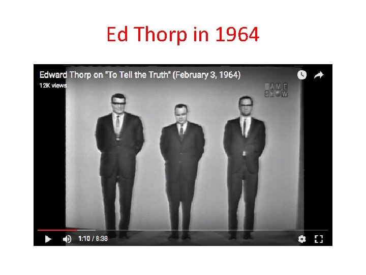
Ed Thorp in 1964

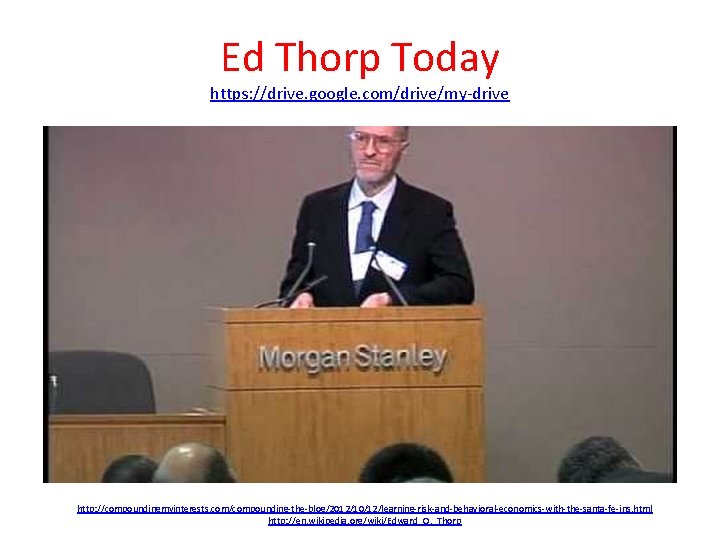
Ed Thorp Today https: //drive. google. com/drive/my-drive http: //compoundingmyinterests. com/compounding-the-blog/2012/10/12/learning-risk-and-behavioral-economics-with-the-santa-fe-ins. html http: //en. wikipedia. org/wiki/Edward_O. _Thorp