27 301 MicrostructureProperties Lecture 1 Microstructure Measurement Profs

27 -301 Microstructure-Properties Lecture 1: Microstructure Measurement Profs. A. D. Rollett, M. De Graef Updated 30 th August, 2015

2 Course Objectives • • • The main objective of this course is to introduce you to the concept of microstructure-property relationships and the power of being able to control material properties through microstructure. Previous courses have given you basic knowledge about microstructure and shown you how to use basic ideas in crystal structure (201), thermodynamics (215), defects (202) and phase relationships (217) in order to understand predict microstructure. Now we will continue on to show you how the properties of materials depend on their microstructure, which allows you to change the properties via controlling microstructure. 301 (this required course) focuses mainly on single-phase materials but with an introduction to composites. 367 (required course) teaches you about materials selection and builds upon all the previous courses. The final stages of the MSE program, e. g. 401, show you how to relate properties (thus microstructure & processing) to design. Please acknowledge Carnegie Mellon if you make public use of these slides

3 Q&A • • Name a pioneer in studying microstructure and • explain what they did. Sorby, for example, cut and polished specimens (esp. of steels) and examined them using optical microscopy. Name a method for measuring grain size and explain it. Reduce an image to lines representing grain boundaries; draw test lines across the image; count the number of intersections per unit length; compute the mean intercept length. Name a second method for measuring grain size and • explain it. Reduce an image to lines representing grain boundaries; count the area belonging to each grain in the image (e. g. by counting pixels), noting whether the grain is complete or touches an edge; compensate for the finite thickness of the boundary lines (if necessary); compute the average area per grain as total area divided by the number of grains (considering edge grains as contributing each ½); compute, if needed, the circle-equivalent radius. Explain the difference between a low angle grain boundary (LAGB) and a high angle grain boundary (HAGB); describe the variation in energy and mobility. A LAGB can be constructed as an array of dislocations; • it has low energy and mobility compared to the HAGB. A HAGB has a disordered atomic structure (and cannot be represented by dislocations because the cores would overlap) with high (constant) energy and mobility. The energy of LAGBs can be described by the Read-Shockley model; for mobility we can use an exponential function. Explain the difference between an analytical property and a complex property. Allowing for this distinction being particular to this course, an analytical property is one that can be described with a linear relationship, and is sometimes calculable from first principles, e. g. elastic modulus. A complex property is one that is generally nonlinear and dependent on the behavior of large populations of defects, e. g. work hardening, e. g. fracture. Explain what is meant by (crystallographic) texture. There is a certain relationship between the crystal axes of each grain and a frame attached to the sample. Any bias in the alignment of crystal axes is called texture. A consequence of texture is that any anisotropy present in the single crystal properties is then present in the polycrystalline material. We use transformation of axes to convert properties known in the crystal frame, for example, to the sample frame. The relationship between single crystal and polycrystal properties may, however, be complex. Explain pole figures and inverse pole figures. A pole figure is a map of a chosen plane normal (pole) with respect to the specimen frame; typically the individual points are binned, smoothed and graphed as a contour plot. An inverse pole figure is the same plot but a chosen sample direction (e. g. the rolling direction) is depicted with respect to the crystal frame. Please acknowledge Carnegie Mellon if you make public use of these slides

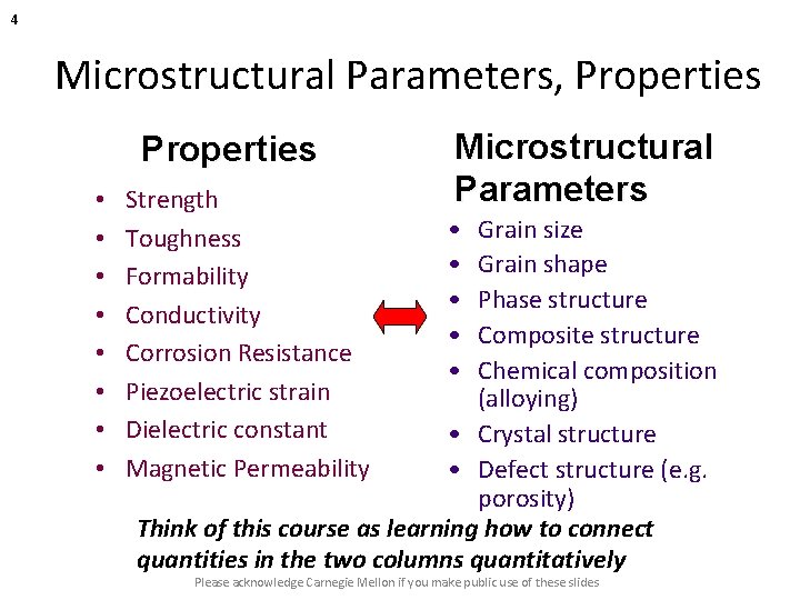
4 Microstructural Parameters, Properties • • Strength Toughness Formability Conductivity Corrosion Resistance Piezoelectric strain Dielectric constant Magnetic Permeability Microstructural Parameters • • • Grain size Grain shape Phase structure Composite structure Chemical composition (alloying) • Crystal structure • Defect structure (e. g. porosity) Think of this course as learning how to connect quantities in the two columns quantitatively Please acknowledge Carnegie Mellon if you make public use of these slides

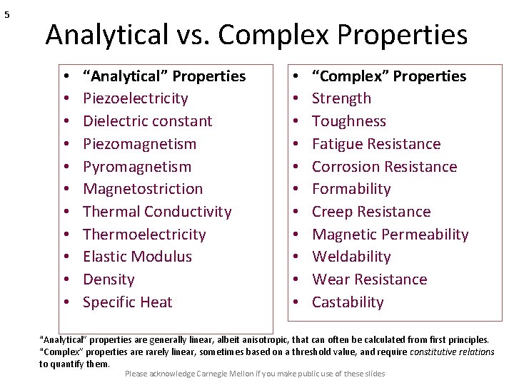
5 Analytical vs. Complex Properties • • • “Analytical” Properties Piezoelectricity Dielectric constant Piezomagnetism Pyromagnetism Magnetostriction Thermal Conductivity Thermoelectricity Elastic Modulus Density Specific Heat • • • “Complex” Properties Strength Toughness Fatigue Resistance Corrosion Resistance Formability Creep Resistance Magnetic Permeability Weldability Wear Resistance Castability “Analytical” properties are generally linear, albeit anisotropic, that can often be calculated from first principles. “Complex” properties are rarely linear, sometimes based on a threshold value, and require constitutive relations to quantify them. Please acknowledge Carnegie Mellon if you make public use of these slides

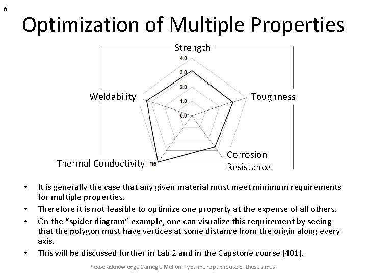
6 Optimization of Multiple Properties Strength Weldability Thermal Conductivity • • Toughness Corrosion Resistance It is generally the case that any given material must meet minimum requirements for multiple properties. Therefore it is not feasible to optimize one property at the expense of all others. On the “spider diagram” example, one can visualize this requirement by seeing that the polygon must have vertices at some distance from the origin along every axis. This will be discussed further in Lab 2 and in the Capstone course (401). Please acknowledge Carnegie Mellon if you make public use of these slides

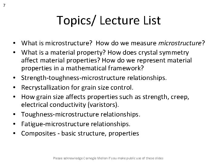
7 Topics/ Lecture List • What is microstructure? How do we measure microstructure? • What is a material property? How does crystal symmetry affect material properties? How do we represent material properties in a mathematical framework? • Strength-toughness-microstructure relationships. • Recrystallization for grain size control. • How grain size affects properties such as strength, creep, electrical conductivity (varistors). • Toughness-microstructure relationships. • Fatigue-microstructure relationships. • Composites - basic structure, properties Please acknowledge Carnegie Mellon if you make public use of these slides

8 Details • All relevant materials for the course are published on the Blackboard website. • CAs for Labs in 301: see the posted Syllabus. • Homework each week, posted on website. • Quiz each week; mostly Wednesdays. • 3 Exams: see the posted Schedule. • Two Labs: Lab 1 on recrystallization+ measurement of microstructure (written report); Lab 2 on mechanical behavior + optimization of properties (oral presentations plus copies of slides with full supplemental information). • Labs will run concurrently (lack of equipment), so consult the Lab groups, schedule. • Computer skills: Excel, Matlab (for homeworks) and Image. J (for image analysis, Labs). • Extensive in-class interaction; reading of lecture notes expected so that we can discuss concepts in class. Please acknowledge Carnegie Mellon if you make public use of these slides

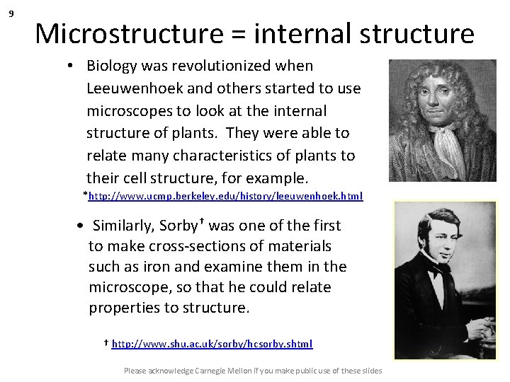
9 Microstructure = internal structure • Biology was revolutionized when Leeuwenhoek and others started to use microscopes to look at the internal structure of plants. They were able to relate many characteristics of plants to their cell structure, for example. *http: //www. ucmp. berkeley. edu/history/leeuwenhoek. html • Similarly, Sorby† was one of the first to make cross-sections of materials such as iron and examine them in the microscope, so that he could relate properties to structure. † http: //www. shu. ac. uk/sorby/hcsorby. shtml Please acknowledge Carnegie Mellon if you make public use of these slides

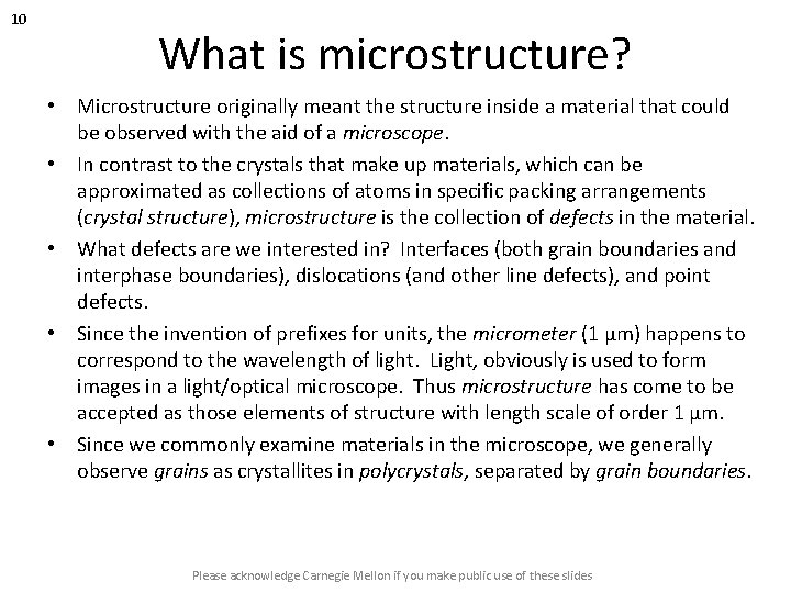
10 What is microstructure? • Microstructure originally meant the structure inside a material that could be observed with the aid of a microscope. • In contrast to the crystals that make up materials, which can be approximated as collections of atoms in specific packing arrangements (crystal structure), microstructure is the collection of defects in the material. • What defects are we interested in? Interfaces (both grain boundaries and interphase boundaries), dislocations (and other line defects), and point defects. • Since the invention of prefixes for units, the micrometer (1 µm) happens to correspond to the wavelength of light. Light, obviously is used to form images in a light/optical microscope. Thus microstructure has come to be accepted as those elements of structure with length scale of order 1 µm. • Since we commonly examine materials in the microscope, we generally observe grains as crystallites in polycrystals, separated by grain boundaries. Please acknowledge Carnegie Mellon if you make public use of these slides

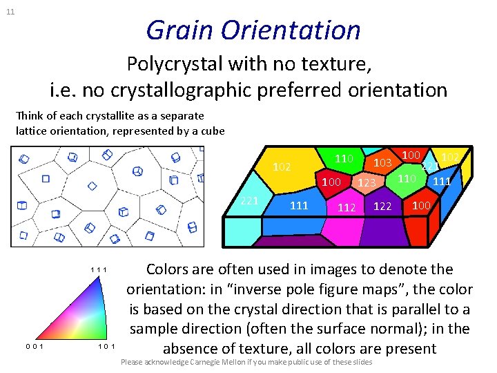
11 Grain Orientation Polycrystal with no texture, i. e. no crystallographic preferred orientation Think of each crystallite as a separate lattice orientation, represented by a cube 102 221 110 103 123 112 122 100 102 221 110 111 100 Colors are often used in images to denote the orientation: in “inverse pole figure maps”, the color is based on the crystal direction that is parallel to a sample direction (often the surface normal); in the absence of texture, all colors are present Please acknowledge Carnegie Mellon if you make public use of these slides

12 Grain Orientation Texture Polycrystal with orientation texture [111] Axial texture: in this example (often observed in rolled sheets of bcc metals), most grains have a <111> // sample normal Grain colors correlate with orientation; here the strong color indicates a strong texture Please acknowledge Carnegie Mellon if you make public use of these slides

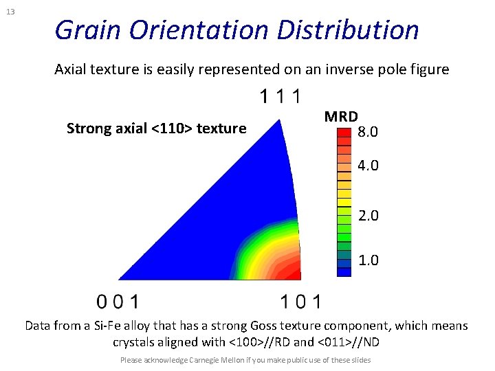
13 Grain Orientation Distribution Axial texture is easily represented on an inverse pole figure Strong axial <110> texture MRD 8. 0 4. 0 2. 0 1. 0 Data from a Si-Fe alloy that has a strong Goss texture component, which means crystals aligned with <100>//RD and <011>//ND Please acknowledge Carnegie Mellon if you make public use of these slides

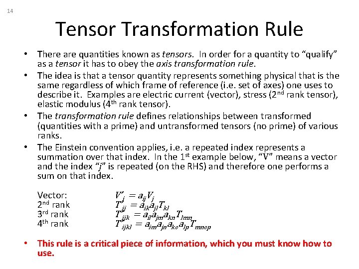
14 Tensor Transformation Rule • There are quantities known as tensors. In order for a quantity to “qualify” as a tensor it has to obey the axis transformation rule. • The idea is that a tensor quantity represents something physical that is the same regardless of which frame of reference (i. e. set of axes) one uses to describe it. Examples are electric current (vector), stress (2 nd rank tensor), elastic modulus (4 th rank tensor). • The transformation rule defines relationships between transformed (quantities with a prime) and untransformed tensors (no prime) of various ranks. • The Einstein convention applies, i. e. a repeated index represents a summation over that index. In the 1 st example below, “V” means a vector and the index “j” is repeated (on the RHS) and therefore one performs a sum on that index. Vector: 2 nd rank 3 rd rank 4 th rank V’i = aij. Vj T’ij = aikajl. Tkl T’ijk = ailajmakn. Tlmn T’ijkl = aimajnakoalp. Tmnop • This rule is a critical piece of information, which you must know how to use.

15 Axis Transformations for Texture • We now define how we use axis transformation to deal with problems involving texture (crystal orientation). • The standard definition of crystal orientation is with an orientation matrix, g, which is exactly equivalent to the “a” on the previous slide. We associate a unit vector, ê, with each axis in both the crystal and the sample reference frames. The orientation matrix is then calculated as follows. gij = êcrystal • êsample • Given any quantity expressed in sample coordinates, it can be transformed (converted, if you like) to crystal coordinates by using the version of the tensor transformation rule that is appropriate to the rank of the tensor concerned (previous slide). • To transform in the opposite direction (crystal to sample), one uses the same transformation but reverses the sense of rotation. This sounds complicated but it’s actually simple because one uses the transpose, g. T. That we can do this is because of the properties of rotations, which can be described by orthogonal matrices. Please acknowledge Carnegie Mellon if you make public use of these slides

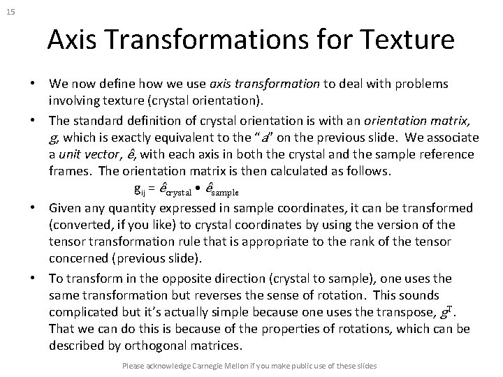
16 Axis Transformation: Examples As a practical illustration, consider where the color in the inverse pole figure map comes from. What we want is to know which crystal axis is parallel to the surface normal of a sample. By convention, we assume a perfectly flat surface and set the sample z-axis perpendicular to the surface (with the x- and y-axes in the plane). • This means that we need to transform a vector, V=[0, 0, 1], where the numbers are the x, y & z coefficients of the vector. (Vectors are 1 st rank tensors). • Using a Matlab routine called Euler. To. Matrix_ADR. m, we can obtain an orientation matrix from a set of three Euler angles (to be explained at a later date), specified as [0. , 54. 5, 45. ]. Orientation Matrix: = --1 --> --2 --> --3 --> --1 --> 0. 70711 0. 41062 0. 57567 --2 --> -0. 70711 0. 41062 0. 57567 --3 --> 0 -0. 81412 0. 58070 • By performing matrix multiplication of this matrix with the vector (treat it as a column vector), V = [0, 0, 1], we obtain the new, transformed vector, V’ = [0. 576, 0. 581]. • In relation to the color maps already shown, this transformed vector is very close to [111], which means that we would color that grain blue. • • Please acknowledge Carnegie Mellon if you make public use of these slides

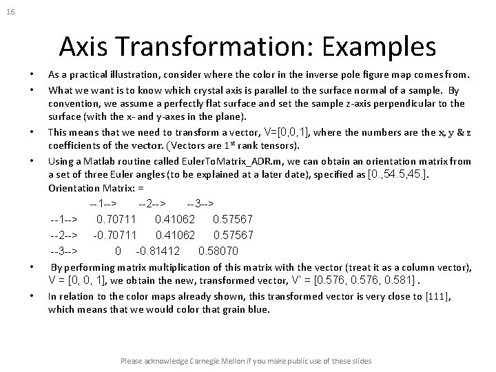
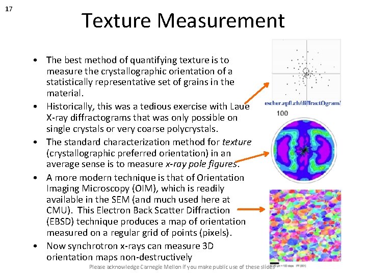
17 Texture Measurement • The best method of quantifying texture is to measure the crystallographic orientation of a statistically representative set of grains in the material. • Historically, this was a tedious exercise with Laue X-ray diffractograms that was only possible on single crystals or very coarse polycrystals. • The standard characterization method for texture (crystallographic preferred orientation) in an average sense is to measure x-ray pole figures. • A more modern technique is that of Orientation Imaging Microscopy (OIM), which is readily available in the SEM (and much used here at CMU). This Electron Back Scatter Diffraction (EBSD) technique produces a map of orientation measured on a regular grid of points (pixels). • Now synchrotron x-rays can measure 3 D orientation maps non-destructively Please acknowledge Carnegie Mellon if you make public use of these slides

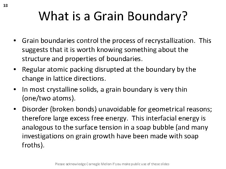
18 What is a Grain Boundary? • Grain boundaries control the process of recrystallization. This suggests that it is worth knowing something about the structure and properties of boundaries. • Regular atomic packing disrupted at the boundary by the change in lattice directions. • In most crystalline solids, a grain boundary is very thin (one/two atoms). • Disorder (broken bonds) unavoidable for geometrical reasons; therefore large excess free energy. This interfacial energy is analogous to the surface tension in a soap bubble (and many investigations on grain growth have been made with soap froths). Please acknowledge Carnegie Mellon if you make public use of these slides

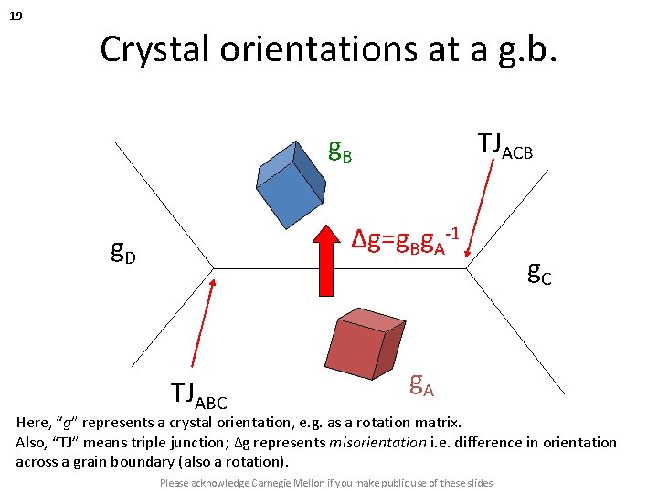
19 Crystal orientations at a g. b. TJACB g. B ∆g=g. Bg. A-1 g. D TJABC g. A Here, “g” represents a crystal orientation, e. g. as a rotation matrix. Also, “TJ” means triple junction; ∆g represents misorientation i. e. difference in orientation across a grain boundary (also a rotation). Please acknowledge Carnegie Mellon if you make public use of these slides

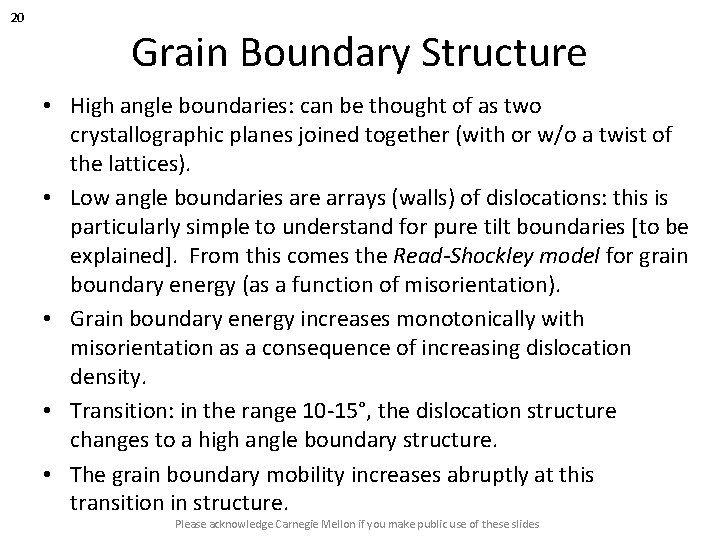
20 Grain Boundary Structure • High angle boundaries: can be thought of as two crystallographic planes joined together (with or w/o a twist of the lattices). • Low angle boundaries are arrays (walls) of dislocations: this is particularly simple to understand for pure tilt boundaries [to be explained]. From this comes the Read-Shockley model for grain boundary energy (as a function of misorientation). • Grain boundary energy increases monotonically with misorientation as a consequence of increasing dislocation density. • Transition: in the range 10 -15°, the dislocation structure changes to a high angle boundary structure. • The grain boundary mobility increases abruptly at this transition in structure. Please acknowledge Carnegie Mellon if you make public use of these slides

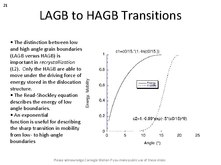
21 LAGB to HAGB Transitions • The distinction between low and high angle grain boundaries (LAGB versus HAGB) is important in recrystallization (L 2). Only the HAGB are able to move under the driving force of energy stored in the dislocation structure. • The Read-Shockley equation describes the energy of low angle boundaries. • An exponential function is useful for describing the sharp transition in mobility from low- to high-angle boundaries Please acknowledge Carnegie Mellon if you make public use of these slides

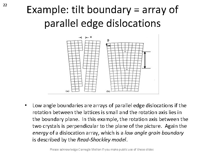
22 Example: tilt boundary = array of parallel edge dislocations b • Low angle boundaries are arrays of parallel edge dislocations if the rotation between the lattices is small and the rotation axis lies in the boundary plane. In this example, the rotation axis between the two crystals is perpendicular to the plane of the picture. Again the energy of a dislocation array, which is a low angle grain boundary is described by the Read-Shockley model. Please acknowledge Carnegie Mellon if you make public use of these slides

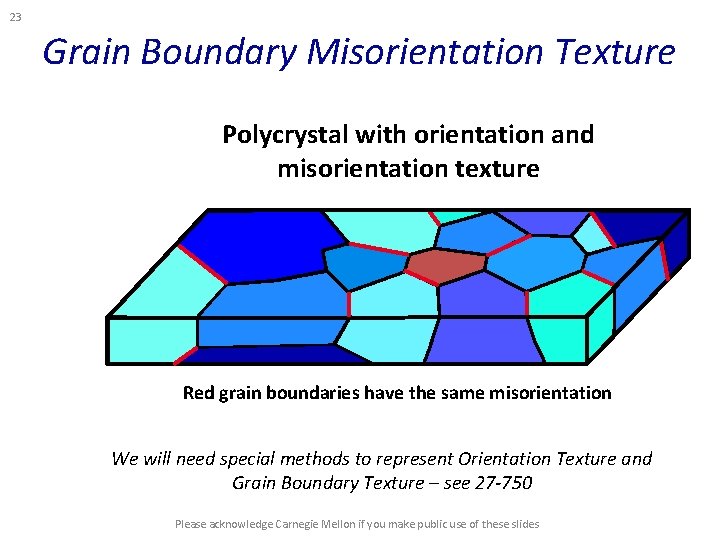
23 Grain Boundary Misorientation Texture Polycrystal with orientation and misorientation texture Red grain boundaries have the same misorientation We will need special methods to represent Orientation Texture and Grain Boundary Texture – see 27 -750 Please acknowledge Carnegie Mellon if you make public use of these slides

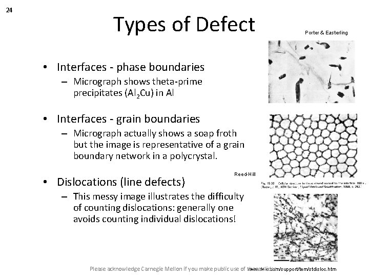
24 Types of Defect Porter & Easterling • Interfaces - phase boundaries – Micrograph shows theta-prime precipitates (Al 2 Cu) in Al • Interfaces - grain boundaries – Micrograph actually shows a soap froth but the image is representative of a grain boundary network in a polycrystal. • Dislocations (line defects) Reed-Hill – This messy image illustrates the difficulty of counting dislocations: generally one avoids counting individual dislocations! www. feic. com/support/tem/stdisloc. htm Please acknowledge Carnegie Mellon if you make public use of these slides

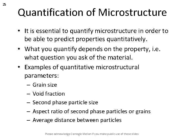
25 Quantification of Microstructure • It is essential to quantify microstructure in order to be able to predict properties quantitatively. • What you quantify depends on the property, i. e. what question you ask of the material. • Examples of quantitative microstructural parameters: – – – Grain size Void fraction Second phase particle size Aspect ratio of second phase particles or grains Average distance between particles Please acknowledge Carnegie Mellon if you make public use of these slides

26 Grain Size Measurement How to measure with linear intercepts How to measure with area counts Grain size number (the E 112 ASTM standard) The problem of plane sections (stereology) The problem of grain shape See: http: //www. metallography. com/grain. htm • Useful references: : Quantitative Stereology, E. E. Underwood, Addison-Wesley, 1970; Practical Stereology by John C. Russ. • • • Please acknowledge Carnegie Mellon if you make public use of these slides

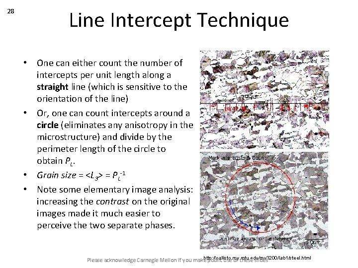
27 Grain size Measurement Linear Intercept Methods • In the case of ‘space-filling’ grains, Stereology provides us with a simple relationship: <L> = 1/NL = 1/PL. • Definitions: <L>: = mean intercept length NL : = number of intercepts per unit length PL : = number of points per unit length • Test lines can be straight or circles depending on method (next page highlights comparison) • Grain shape determines whether the mean intercept length, <L>, is a 2 D or 3 D parameter. Equiaxed <L 3> Columnar <L 2> Why? Area-based Method (Planimetric Method) • Another simple measure of grain size in 2 D sections is based on area. Count the number of grains, NA, and also measure the area in the image (an edge grain is counted as 0. 5). Divide the area by the number to obtain <A>. One may then calculate the areaequivalent diameter (or circle-equivalent diameter), <D> = 2√(<A>/π). • This approach can only be applied to equiaxed morphologies! Slight deviations from equiaxed lead to significant errors in the estimated grain size. This size, <D>, is not the same as the mean intercept length, <L>! Please acknowledge Carnegie Mellon if you make public use of these slides

28 Line Intercept Technique • One can either count the number of intercepts per unit length along a straight line (which is sensitive to the orientation of the line) • Or, one can count intercepts around a circle (eliminates any anisotropy in the microstructure) and divide by the perimeter length of the circle to obtain PL. • Grain size = <L 3> = PL-1 • Note some elementary image analysis: increasing the contrast on the original images made it much easier to perceive the two separate phases. Please acknowledge Carnegie Mellon if you makehttp: //callisto. my. mtu. edu/my 3200/lab 1/steel. html public use of these slides

29 Grain size measurement: intercepts • From Table 2. 2 [Underwood], column (a), illustrates how to make a measurement of the mean intercept length, based on the number of grains per unit length of test line. <L 3> = 1/NL • Important: use many test lines that are randomly oriented with respect to the structure. • Assuming spherical† grains, <L 3> = 4 r/3, [Underwood, Table 4. 1], there are 7 intersections and if we take the total (red) test line length, LT= 798µm, then LTNL= 7, so NL= 1/114 µm-1 d = 2*3*<L 3>/4 = 6/(4*NL) = 6*114/4 = 171 µm. † Ask yourself what a better assumption about grain shape might be! Please acknowledge Carnegie Mellon if you make public use of these slides

30 Grain size measurement: area based [Underwood] Fig. 7. 12 • Grain count method: <A>=1/NA • Number of whole grains= 20 Number of edge grains= 21 Effective total=Nwhole+Nedge/2 = 30. 5 Total area= 0. 5 mm 2 Thus, NA= 61 mm-2; <A>=16, 400 µm 2 2 D size: d = 2√(<A>/π) = 177 µm. • For 3 D, assume spherical grains, <A> mean intercept area= 2/3πr 2 d = 2√(3<A>/2π)= 144 µm. • Neither of these values is equal to the value determined on the previous slide, using the linear intercept method. Please acknowledge Carnegie Mellon if you make public use of these slides

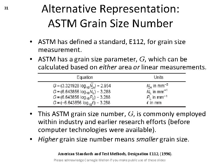
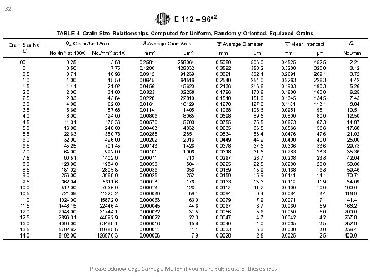
31 Alternative Representation: ASTM Grain Size Number • ASTM has defined a standard, E 112, for grain size measurement. • ASTM has a grain size parameter, G, which can be calculated based on either area or linear measurements. • This ASTM grain size number, G, is commonly employed within industry and earlier research efforts (before computer technologies were available). • Higher grain size number means smaller grain size. American Standards and Test Methods, Designation E 112, (1996). Please acknowledge Carnegie Mellon if you make public use of these slides

32 Please acknowledge Carnegie Mellon if you make public use of these slides

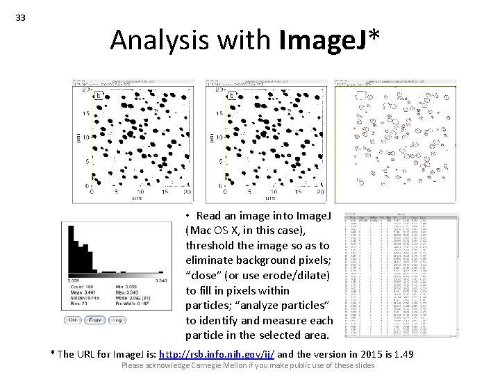
33 Analysis with Image. J* • Read an image into Image. J (Mac OS X, in this case), threshold the image so as to eliminate background pixels; “close” (or use erode/dilate) to fill in pixels within particles; “analyze particles” to identify and measure each particle in the selected area. * The URL for Image. J is: http: //rsb. info. nih. gov/ij/ and the version in 2015 is 1. 49 Please acknowledge Carnegie Mellon if you make public use of these slides

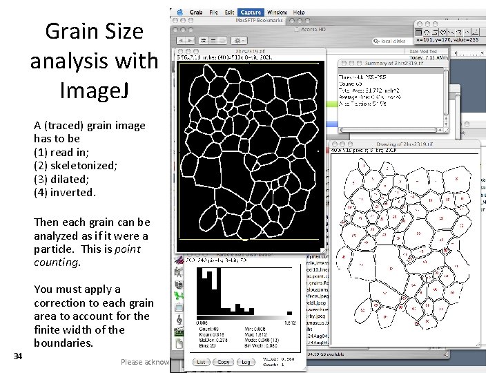
Grain Size analysis with Image. J A (traced) grain image has to be (1) read in; (2) skeletonized; (3) dilated; (4) inverted. Then each grain can be analyzed as if it were a particle. This is point counting. 34 You must apply a correction to each grain area to account for the finite width of the boundaries. Please acknowledge Carnegie Mellon if you make public use of these slides

35 Recommended • • • • Books, References Porter, D. A. & K. E. Easterling, Phase transformations in metals and alloys, Chapman & Hall (669. 94 P 84 P 2) Newnham, R. E. , Properties of Materials: Anisotropy, Symmetry, Structure. Oxford University Press, 2004. Nye, J. F. , Physical Properties of Crystals. Clarendon Press, 1957 (548. 8 N 99 PA); this book has been reprinted fairly recently. Underwood, E. E. , Quantitative Stereology, 1971, Addison-Wesley Humphreys, F. J. and M. Hatherly (1996). Recrystallization and related annealing phenomena. Oxford, UK, Elsevier Science, Oxford, UK Russ, J. C. and R. T. Dehoff (1999). Practical Stereology, New York, Plenum Press. Reed-Hill, R. E. (1973). Physical Metallurgy Principles, New York, Van Nostrand. http: //www. metallography. com/grain. htm - grain size measurement http: //www. stereologysociety. org/ - resources for stereology http: //www. doitpoms. ac. uk/ - a nice library of micrographs and microstructures at the Univ. Cambridge (UK) Howard, C. V. and M. G. Reed (1998). Unbiased Stereology, New York, Springer-Verlag. Martin, J. , R. D. Doherty, et al. (1997). Stability of microstructure in metallic systems. Cambridge, England, Cambridge University Press. Nutting & Baker, The Microstructure of Metals, 1965, The Institute of Metals (UK). Please acknowledge Carnegie Mellon if you make public use of these slides

36 Summary • Objectives of the course have been described. • Examples of ‘typical’ microstructures described. • Methods for measuring grain size described: first method is based on linear intercepts. Second method is based on average area on the cross section. Please acknowledge Carnegie Mellon if you make public use of these slides

37 Supplemental Slides • The following slides provide supplemental information, e. g. to explain what stereology is. Please acknowledge Carnegie Mellon if you make public use of these slides

38 Plane sectioning • General problem: how can one estimate the true 3 D distribution of sizes based on (2 D) plane sections through the objects? This challenge is the essence of stereology. • Imagine an array of spheres randomly arranged in space: cut through the space with a plane: examine the spheres. What do you see? • Answer: a array of circles of variable size, of which the maximum possible diameter (size) is the sphere diameter. • How to measure? The easiest is to draw random straight lines and measure intercepts. Please acknowledge Carnegie Mellon if you make public use of these slides

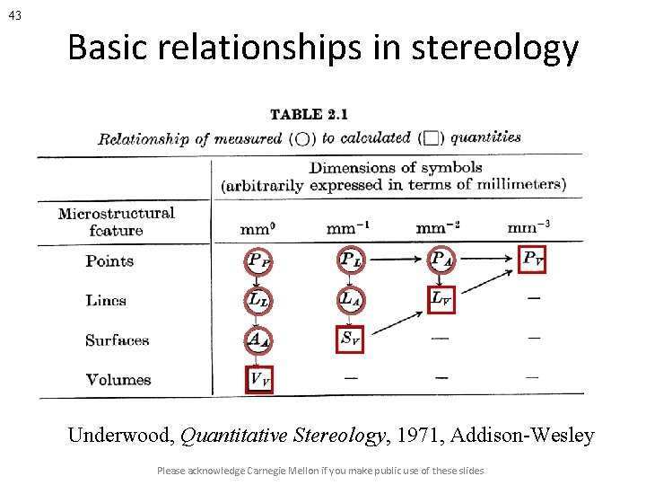
39 Stereology • Stereology provides us with relationships between quantities that are measurable on a plane section, and 3 D quantities that we may need. • Two quantities that are (relatively) easily measured are the number of points per unit length along a line, PL, and the number of points per unit area, PA. This nomenclature can be extended to volumes (V) and surfaces (S). • Quantities per unit volume have to be calculated (table). • In this course, we will describe a few key results from stereology, mainly motivated by the need to be able to measure grain size. No derivations of the equations will be carried out. Please acknowledge Carnegie Mellon if you make public use of these slides

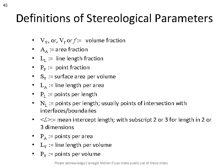
40 Definitions of Stereological Parameters • • • VV, or, Vf or f : = volume fraction AA : = area fraction LL : = line length fraction PP : = point fraction SV : = surface area per volume LA : = line length per area PL : = points per length NL : = points per length; usually points of intersection with interfaces/boundaries <L>: = mean intercept length; with subscript 2 or 3 for length in 2 or 3 dimensions PA : = points per area LV : = line length per volume PV : = points per volume Please acknowledge Carnegie Mellon if you make public use of these slides

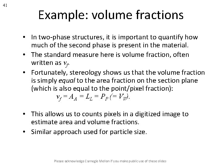
41 Example: volume fractions • In two-phase structures, it is important to quantify how much of the second phase is present in the material. • The standard measure here is volume fraction, often written as vf. • Fortunately, stereology shows us that the volume fraction is simply equal to the area fraction on the section plane (which is also equal to the point/pixel fraction): vf = AA = LL = PP (= VV). • This allows us to counts pixels in a digitized image to estimate area and volume fractions. • Similar approach used for particle size. Please acknowledge Carnegie Mellon if you make public use of these slides

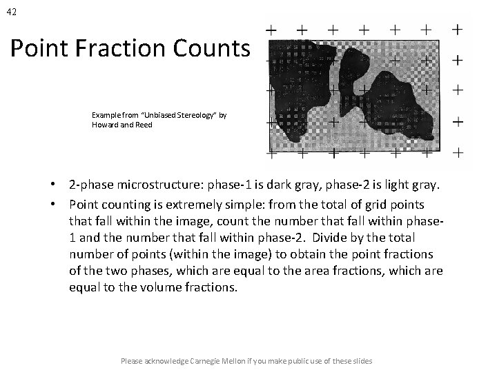
42 Point Fraction Counts Example from “Unbiased Stereology” by Howard and Reed • 2 -phase microstructure: phase-1 is dark gray, phase-2 is light gray. • Point counting is extremely simple: from the total of grid points that fall within the image, count the number that fall within phase 1 and the number that fall within phase-2. Divide by the total number of points (within the image) to obtain the point fractions of the two phases, which are equal to the area fractions, which are equal to the volume fractions. Please acknowledge Carnegie Mellon if you make public use of these slides

43 Basic relationships in stereology Underwood, Quantitative Stereology, 1971, Addison-Wesley Please acknowledge Carnegie Mellon if you make public use of these slides

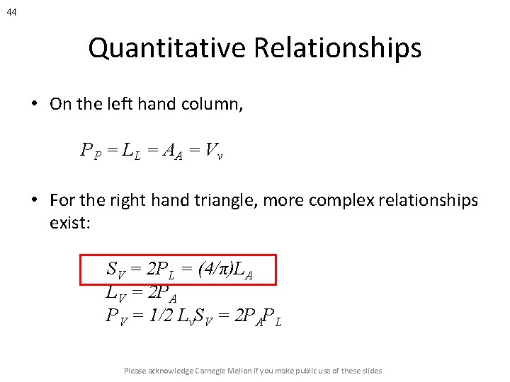
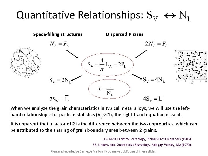
44 Quantitative Relationships • On the left hand column, PP = LL = A A = V v • For the right hand triangle, more complex relationships exist: SV = 2 PL = (4/π)LA LV = 2 PA PV = 1/2 Lv. SV = 2 PAPL Please acknowledge Carnegie Mellon if you make public use of these slides

Quantitative Relationships: SV NL Space-filling structures Dispersed Phases When we analyze the grain characteristics in typical metal alloys, we will use the lefthand relationships; for particle statistics (VV<<1), the right-hand equation is valid. It is apparent that a factor of 2 is the difference between the two approaches, which can be attributed to the sharing of grain boundary area between 2 grains. J. C. Russ, Practical Stereology, Plenum Press, New York (1986). E. E. Underwood, Quantitative Stereology, Addison-Wesley, MA (1970). 45 Please acknowledge Carnegie Mellon if you make public use of these slides

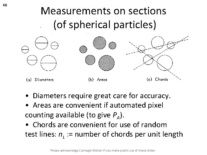
46 Measurements on sections (of spherical particles) • Diameters require great care for accuracy. • Areas are convenient if automated pixel counting available (to give PA). • Chords are convenient for use of random test lines: n. L : = number of chords per unit length Please acknowledge Carnegie Mellon if you make public use of these slides

47 Mean free path, l, versus Nearest neighbor spacing, ∆ • It is useful (and therefore important) to keep the difference between mean free path and nearest neighbor spacing separate and distinct. • Mean free path is how far, on average, you travel from one particle until you encounter another one. • Nearest neighbor spacing is how far apart, on average, two nearest neighbors are from each other. • They appear at first glance to be the same thing but they are not! • They are related to one another, as we shall see in the next few slides. Please acknowledge Carnegie Mellon if you make public use of these slides

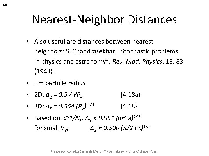
48 Nearest-Neighbor Distances • Also useful are distances between nearest neighbors: S. Chandrasekhar, “Stochastic problems in physics and astronomy”, Rev. Mod. Physics, 15, 83 (1943). • r : = particle radius • 2 D: ∆2 = 0. 5 / √PA (4. 18 a) • 3 D: ∆3 = 0. 554 (PV)-1/3 (4. 18) • Based on l~1/NL, ∆3 0. 554 (πr 2 l)1/3 for small VV, ∆2 0. 500 (π/2 rl)1/2 Please acknowledge Carnegie Mellon if you make public use of these slides

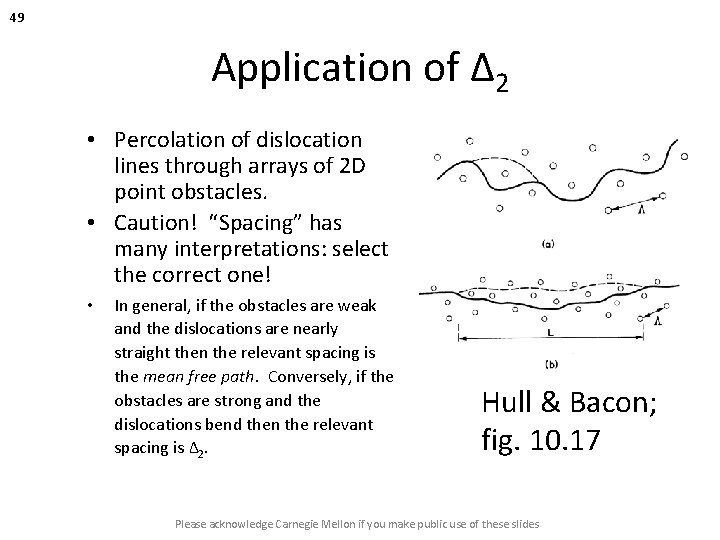
49 Application of ∆2 • Percolation of dislocation lines through arrays of 2 D point obstacles. • Caution! “Spacing” has many interpretations: select the correct one! • In general, if the obstacles are weak and the dislocations are nearly straight then the relevant spacing is the mean free path. Conversely, if the obstacles are strong and the dislocations bend then the relevant spacing is ∆2. Hull & Bacon; fig. 10. 17 Please acknowledge Carnegie Mellon if you make public use of these slides

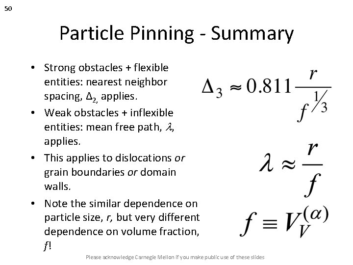
50 Particle Pinning - Summary • Strong obstacles + flexible entities: nearest neighbor spacing, ∆2, applies. • Weak obstacles + inflexible entities: mean free path, l, applies. • This applies to dislocations or grain boundaries or domain walls. • Note the similar dependence on particle size, r, but very different dependence on volume fraction, f! Please acknowledge Carnegie Mellon if you make public use of these slides

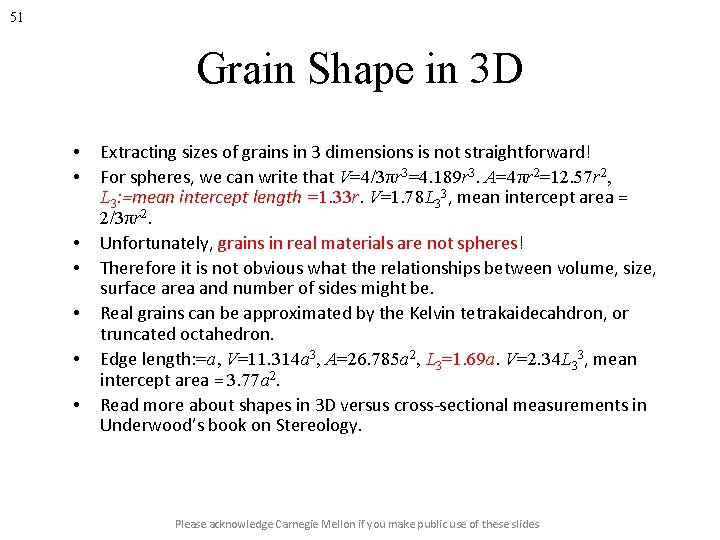
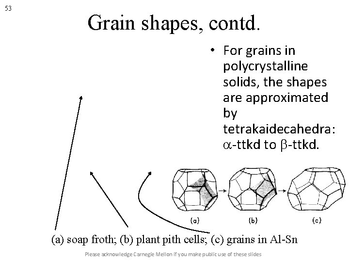
51 Grain Shape in 3 D • • Extracting sizes of grains in 3 dimensions is not straightforward! For spheres, we can write that V=4/3πr 3=4. 189 r 3. A=4πr 2=12. 57 r 2, L 3: =mean intercept length =1. 33 r. V=1. 78 L 33, mean intercept area = 2/3πr 2. Unfortunately, grains in real materials are not spheres! Therefore it is not obvious what the relationships between volume, size, surface area and number of sides might be. Real grains can be approximated by the Kelvin tetrakaidecahdron, or truncated octahedron. Edge length: =a, V=11. 314 a 3, A=26. 785 a 2, L 3=1. 69 a. V=2. 34 L 33, mean intercept area = 3. 77 a 2. Read more about shapes in 3 D versus cross-sectional measurements in Underwood’s book on Stereology. Please acknowledge Carnegie Mellon if you make public use of these slides

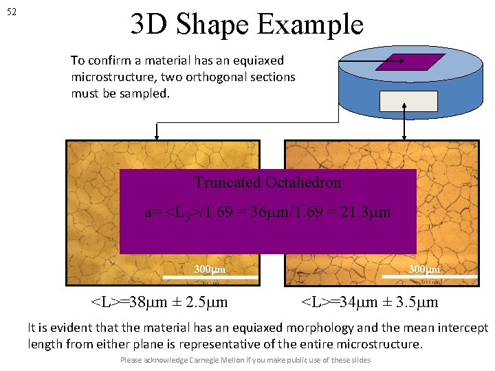
52 3 D Shape Example To confirm a material has an equiaxed microstructure, two orthogonal sections must be sampled. Truncated Octahedron a= <L 3>/1. 69 = 36 mm/1. 69 = 21. 3 mm 300 mm <L>=38 mm ± 2. 5 mm <L>=34 mm ± 3. 5 mm It is evident that the material has an equiaxed morphology and the mean intercept length from either plane is representative of the entire microstructure. Please acknowledge Carnegie Mellon if you make public use of these slides

53 Grain shapes, contd. • For grains in polycrystalline solids, the shapes are approximated by tetrakaidecahedra: a-ttkd to b-ttkd. (a) soap froth; (b) plant pith cells; (c) grains in Al-Sn Please acknowledge Carnegie Mellon if you make public use of these slides

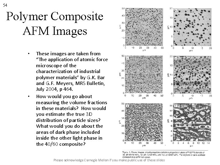
54 Polymer Composite AFM Images • • These images are taken from “The application of atomic force microscope of the characterization of industrial polymer materials” by G. K. Bar and G. F. Meyers, MRS Bulletin, July 2004, p 464. How would you go about measuring the volume fractions in these materials? How would you estimate the true 3 D distribution of particle sizes? What would you do about the areas of dark phase included inside the other light phase in the 40/60 composite? Please acknowledge Carnegie Mellon if you make public use of these slides