27 301 MicrostructureProperties Tensors and Anisotropy Part 2

27 -301 Microstructure-Properties Tensors and Anisotropy, Part 2 Profs. A. D. Rollett, M. De Graef Processing Performance Microstructure Properties Last modified: 15 th Nov. ‘ 15

2 Objective • The objective of this lecture is to explain the meaning of analytical material properties and how to describe their anisotropy. • We show to account for the effect of crystal symmetry on (tensor) material properties. • We motivate the study of anisotropic properties with examples of applications. Please acknowledge Carnegie Mellon in any public use of these slides

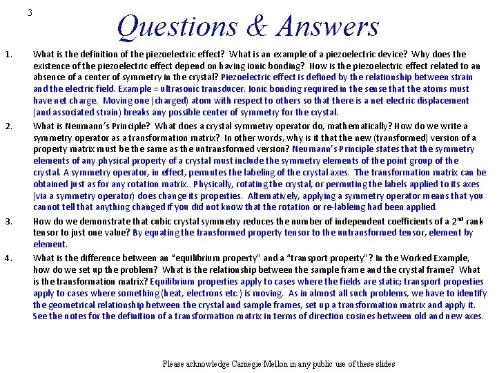
3 1. 2. 3. 4. Questions & Answers What is the definition of the piezoelectric effect? What is an example of a piezoelectric device? Why does the existence of the piezoelectric effect depend on having ionic bonding? How is the piezoelectric effect related to an absence of a center of symmetry in the crystal? Piezoelectric effect is defined by the relationship between strain and the electric field. Example = ultrasonic transducer. Ionic bonding required in the sense that the atoms must have net charge. Moving one (charged) atom with respect to others so that there is a net electric displacement (and associated strain) breaks any possible center of symmetry for the crystal. What is Neumann’s Principle? What does a crystal symmetry operator do, mathematically? How do we write a symmetry operator as a transformation matrix? In other words, why is it that the new (transformed) version of a property matrix must be the same as the untransformed version? Neumann’s Principle states that the symmetry elements of any physical property of a crystal must include the symmetry elements of the point group of the crystal. A symmetry operator, in effect, permutes the labeling of the crystal axes. The transformation matrix can be obtained just as for any rotation matrix. Physically, rotating the crystal, or permuting the labels applied to its axes (via a symmetry operator) does change its properties. Alternatively, applying a symmetry operator means that you cannot tell that anything changed if you did not know that the rotation or re-lableing had been applied. How do we demonstrate that cubic crystal symmetry reduces the number of independent coefficients of a 2 nd rank tensor to just one value? By equating the transformed property tensor to the untransformed tensor, element by element. What is the difference between an “equilibrium property” and a “transport property”? In the Worked Example, how do we set up the problem? What is the relationship between the sample frame and the crystal frame? What is the transformation matrix? Equilibrium properties apply to cases where the fields are static; transport properties apply to cases where something (heat, electrons etc. ) is moving. As in almost all such problems, we have to identify the geometrical relationship between the crystal and sample frames, set up a transformation matrix and apply it. See the notes for the definition of a transformation matrix in terms of direction cosines between old and new axes. Please acknowledge Carnegie Mellon in any public use of these slides

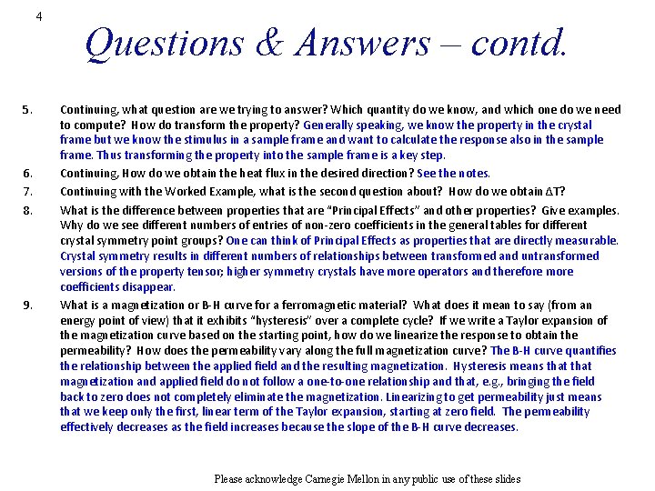
4 5. 6. 7. 8. 9. Questions & Answers – contd. Continuing, what question are we trying to answer? Which quantity do we know, and which one do we need to compute? How do transform the property? Generally speaking, we know the property in the crystal frame but we know the stimulus in a sample frame and want to calculate the response also in the sample frame. Thus transforming the property into the sample frame is a key step. Continuing, How do we obtain the heat flux in the desired direction? See the notes. Continuing with the Worked Example, what is the second question about? How do we obtain ∆T? What is the difference between properties that are “Principal Effects” and other properties? Give examples. Why do we see different numbers of entries of non-zero coefficients in the general tables for different crystal symmetry point groups? One can think of Principal Effects as properties that are directly measurable. Crystal symmetry results in different numbers of relationships between transformed and untransformed versions of the property tensor; higher symmetry crystals have more operators and therefore more coefficients disappear. What is a magnetization or B-H curve for a ferromagnetic material? What does it mean to say (from an energy point of view) that it exhibits “hysteresis” over a complete cycle? If we write a Taylor expansion of the magnetization curve based on the starting point, how do we linearize the response to obtain the permeability? How does the permeability vary along the full magnetization curve? The B-H curve quantifies the relationship between the applied field and the resulting magnetization. Hysteresis means that magnetization and applied field do not follow a one-to-one relationship and that, e. g. , bringing the field back to zero does not completely eliminate the magnetization. Linearizing to get permeability just means that we keep only the first, linear term of the Taylor expansion, starting at zero field. The permeability effectively decreases as the field increases because the slope of the B-H curve decreases. Please acknowledge Carnegie Mellon in any public use of these slides

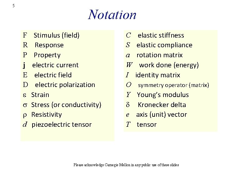
5 Notation F R P j E D e s r d Stimulus (field) Response Property electric current electric field electric polarization Strain Stress (or conductivity) Resistivity piezoelectric tensor C S a W I O Y d e T elastic stiffness elastic compliance rotation matrix work done (energy) identity matrix symmetry operator (matrix) Young’s modulus Kronecker delta axis (unit) vector tensor Please acknowledge Carnegie Mellon in any public use of these slides

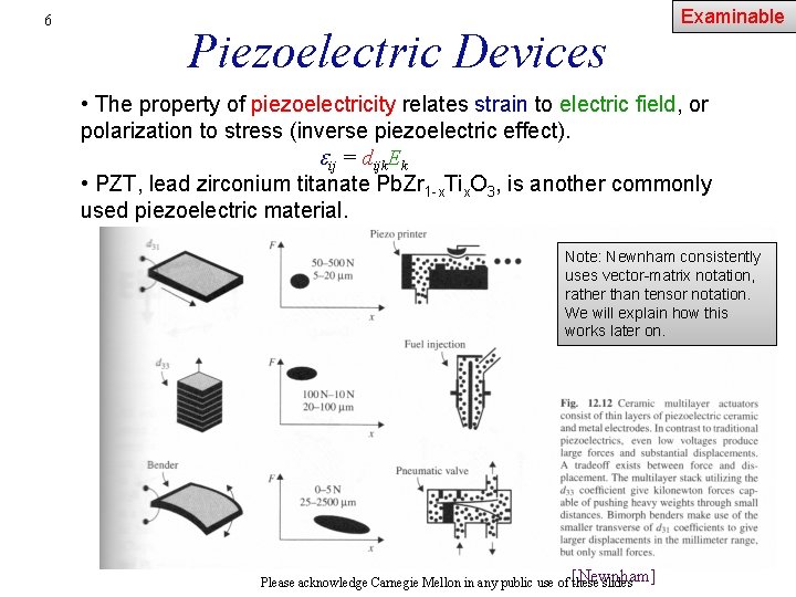
6 Piezoelectric Devices Examinable • The property of piezoelectricity relates strain to electric field, or polarization to stress (inverse piezoelectric effect). ij = dijk. Ek • PZT, lead zirconium titanate Pb. Zr 1 -x. Tix. O 3, is another commonly used piezoelectric material. Note: Newnham consistently uses vector-matrix notation, rather than tensor notation. We will explain how this works later on. Please acknowledge Carnegie Mellon in any public use of [Newnham] these slides

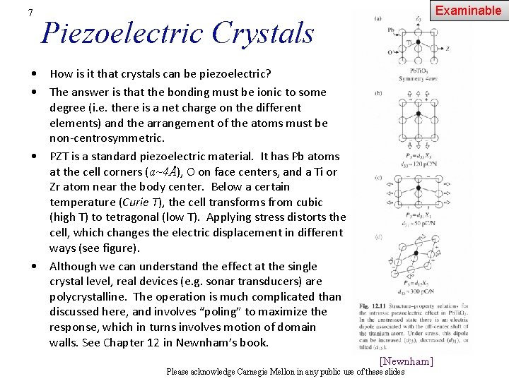
7 Examinable Piezoelectric Crystals • How is it that crystals can be piezoelectric? • The answer is that the bonding must be ionic to some degree (i. e. there is a net charge on the different elements) and the arrangement of the atoms must be non-centrosymmetric. • PZT is a standard piezoelectric material. It has Pb atoms at the cell corners (a~4Å), O on face centers, and a Ti or Zr atom near the body center. Below a certain temperature (Curie T), the cell transforms from cubic (high T) to tetragonal (low T). Applying stress distorts the cell, which changes the electric displacement in different ways (see figure). • Although we can understand the effect at the single crystal level, real devices (e. g. sonar transducers) are polycrystalline. The operation is much complicated than discussed here, and involves “poling” to maximize the response, which in turns involves motion of domain walls. See Chapter 12 in Newnham’s book. [Newnham] Please acknowledge Carnegie Mellon in any public use of these slides

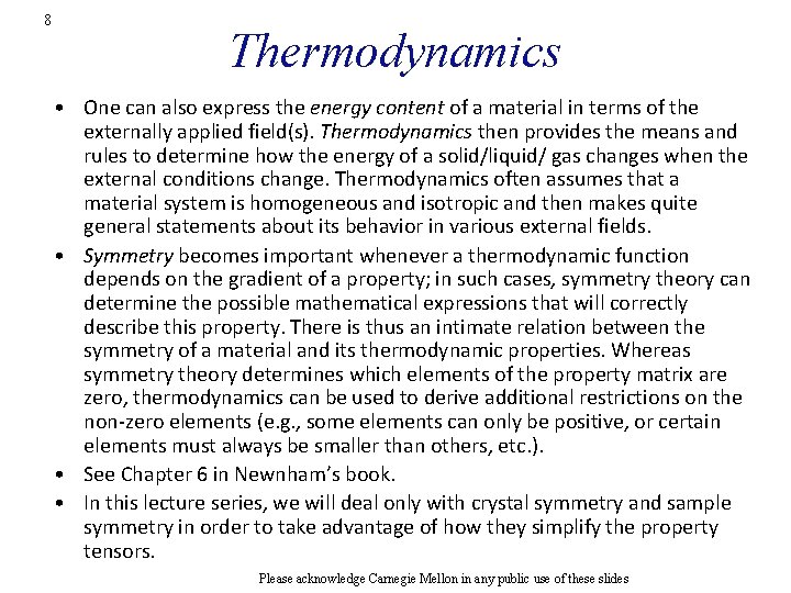
8 Thermodynamics • One can also express the energy content of a material in terms of the externally applied field(s). Thermodynamics then provides the means and rules to determine how the energy of a solid/liquid/ gas changes when the external conditions change. Thermodynamics often assumes that a material system is homogeneous and isotropic and then makes quite general statements about its behavior in various external fields. • Symmetry becomes important whenever a thermodynamic function depends on the gradient of a property; in such cases, symmetry theory can determine the possible mathematical expressions that will correctly describe this property. There is thus an intimate relation between the symmetry of a material and its thermodynamic properties. Whereas symmetry theory determines which elements of the property matrix are zero, thermodynamics can be used to derive additional restrictions on the non-zero elements (e. g. , some elements can only be positive, or certain elements must always be smaller than others, etc. ). • See Chapter 6 in Newnham’s book. • In this lecture series, we will deal only with crystal symmetry and sample symmetry in order to take advantage of how they simplify the property tensors. Please acknowledge Carnegie Mellon in any public use of these slides

9 Neumann's Principle Examinable • A fundamental natural law: Neumann's Principle: the symmetry elements of any physical property of a crystal must include the symmetry elements of the point group of the crystal. The property may have additional symmetry elements to those of the crystal (point group) symmetry. There are 32 crystal classes for the point group symmetry. • Franz Neumann (1795 -1898)'s principle was first stated in his course at the university of Königsberg (1973/1974) and was published in the printed version of his lecture notes (Neumann F. E. , 1885, Vorlesungen über die Theorie der Elastizität der festen Körper und des Lichtäthers, edited by O. E. Meyer. Leipzig, B. G. Teubner-Verlag. [http: //reference. iucr. org/dictionary/Neumann%27 s_principle] • Curie further developed the concepts of how crystal symmetry affects materials properties. Please acknowledge Carnegie Mellon in any public use of these slides

10 Neumann, extended Examinable If a crystal has a defect structure such as a dislocation network that is arranged in a non-uniform way then the symmetry of certain properties may be reduced from the crystal symmetry. In principle, a finite elastic strain in one direction decreases the symmetry of a cubic crystal to tetragonal or less. Therefore the modified version of Neumann's Principle: the symmetry elements of any physical property of a crystal must include the symmetry elements that are common to the point group of the crystal and the defect structure contained within the crystal. Please acknowledge Carnegie Mellon in any public use of these slides

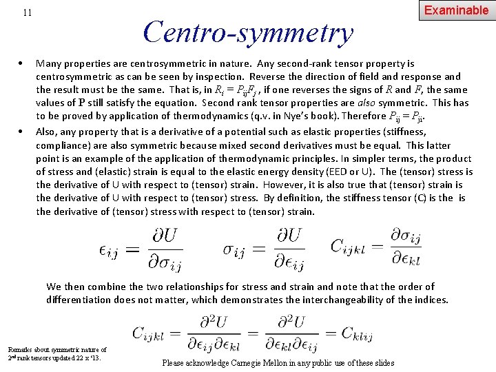
11 • • Centro-symmetry Examinable Many properties are centrosymmetric in nature. Any second-rank tensor property is centrosymmetric as can be seen by inspection. Reverse the direction of field and response and the result must be the same. That is, in Ri = Pij. Fj , if one reverses the signs of R and F, the same values of P still satisfy the equation. Second rank tensor properties are also symmetric. This has to be proved by application of thermodynamics (q. v. in Nye’s book). Therefore Pij = Pji. Also, any property that is a derivative of a potential such as elastic properties (stiffness, compliance) are also symmetric because mixed second derivatives must be equal. This latter point is an example of the application of thermodynamic principles. In simpler terms, the product of stress and (elastic) strain is equal to the elastic energy density (EED or U). The (tensor) stress is the derivative of U with respect to (tensor) strain. However, it is also true that (tensor) strain is the derivative of U with respect to (tensor) stress. By definition, the stiffness tensor (C) is the derivative of (tensor) stress with respect to (tensor) strain. We then combine the two relationships for stress and strain and note that the order of differentiation does not matter, which demonstrates the interchangeability of the indices. Remarks about symmetric nature of 2 nd rank tensors updated 22 x ‘ 13. Please acknowledge Carnegie Mellon in any public use of these slides

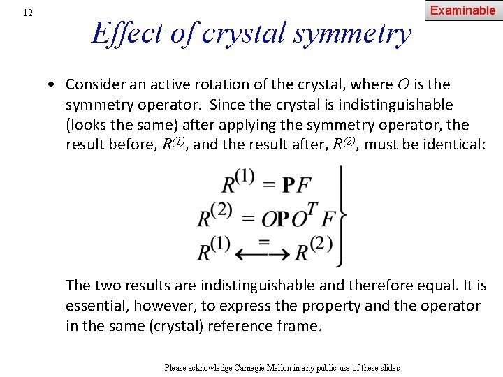
12 Effect of crystal symmetry Examinable • Consider an active rotation of the crystal, where O is the symmetry operator. Since the crystal is indistinguishable (looks the same) after applying the symmetry operator, the result before, R(1), and the result after, R(2), must be identical: The two results are indistinguishable and therefore equal. It is essential, however, to express the property and the operator in the same (crystal) reference frame. Please acknowledge Carnegie Mellon in any public use of these slides

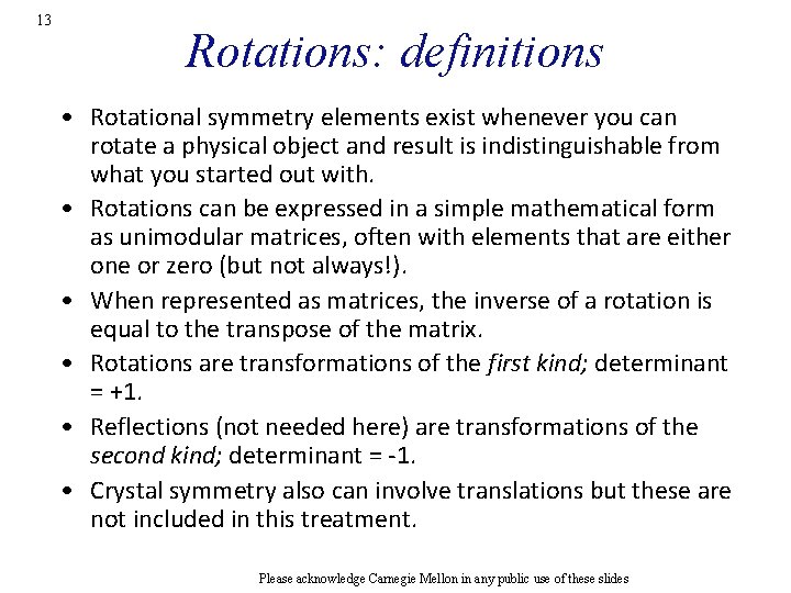
13 Rotations: definitions • Rotational symmetry elements exist whenever you can rotate a physical object and result is indistinguishable from what you started out with. • Rotations can be expressed in a simple mathematical form as unimodular matrices, often with elements that are either one or zero (but not always!). • When represented as matrices, the inverse of a rotation is equal to the transpose of the matrix. • Rotations are transformations of the first kind; determinant = +1. • Reflections (not needed here) are transformations of the second kind; determinant = -1. • Crystal symmetry also can involve translations but these are not included in this treatment. Please acknowledge Carnegie Mellon in any public use of these slides

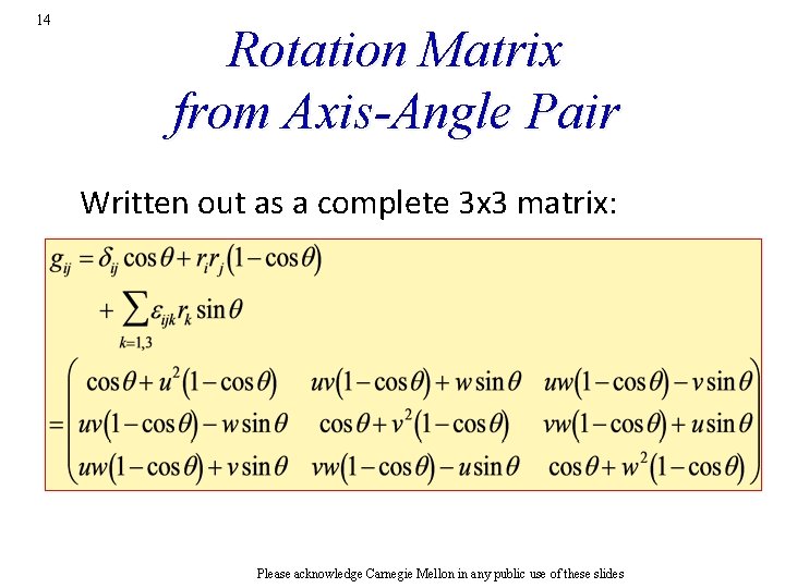
14 Rotation Matrix from Axis-Angle Pair Written out as a complete 3 x 3 matrix: Please acknowledge Carnegie Mellon in any public use of these slides

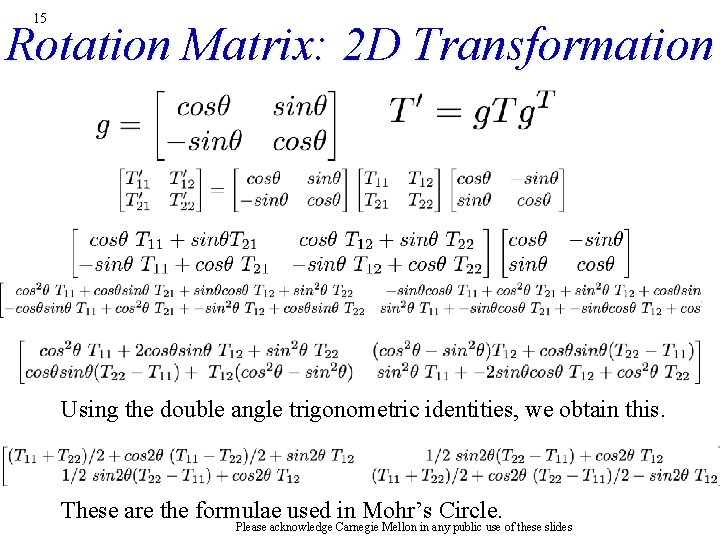
15 Rotation Matrix: 2 D Transformation Using the double angle trigonometric identities, we obtain this. These are the formulae used in Mohr’s Circle. Please acknowledge Carnegie Mellon in any public use of these slides

16 Symmetry Operator examples • Diad on z: [uvw] = [001], = 180° ; substitute the values of uvw and angle into the formula • 4 -fold rotation about x: [uvw] = [100] = 90° Please acknowledge Carnegie Mellon in any public use of these slides

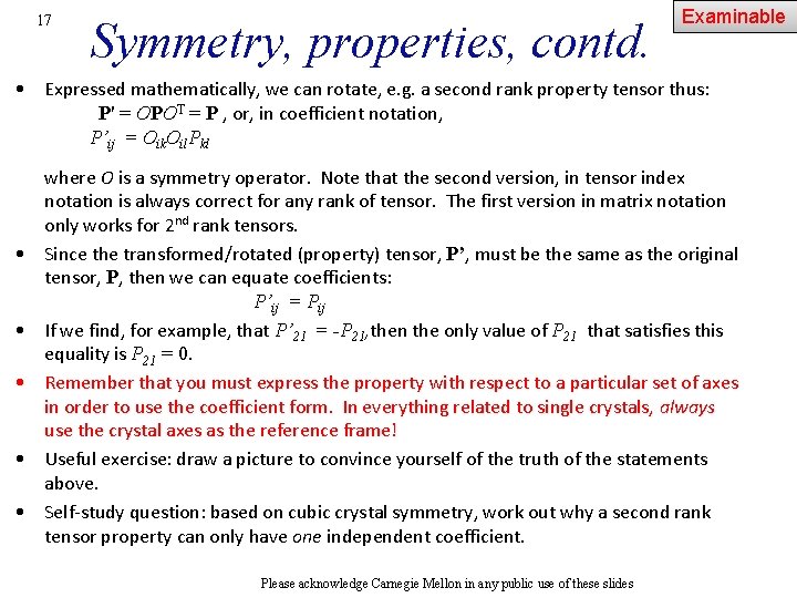
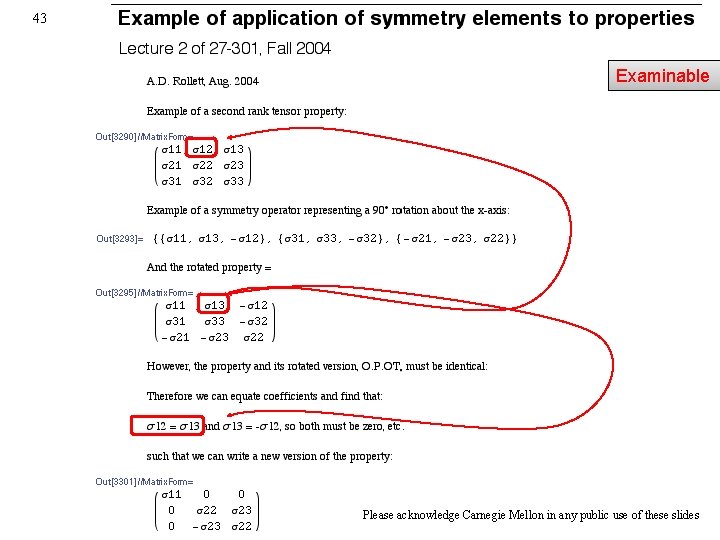
17 Symmetry, properties, contd. Examinable • Expressed mathematically, we can rotate, e. g. a second rank property tensor thus: P' = OPOT = P , or, in coefficient notation, P’ij = Oik. Oil. Pkl • • • where O is a symmetry operator. Note that the second version, in tensor index notation is always correct for any rank of tensor. The first version in matrix notation only works for 2 nd rank tensors. Since the transformed/rotated (property) tensor, P’, must be the same as the original tensor, P, then we can equate coefficients: P’ij = Pij If we find, for example, that P’ 21 = -P 21, then the only value of P 21 that satisfies this equality is P 21 = 0. Remember that you must express the property with respect to a particular set of axes in order to use the coefficient form. In everything related to single crystals, always use the crystal axes as the reference frame! Useful exercise: draw a picture to convince yourself of the truth of the statements above. Self-study question: based on cubic crystal symmetry, work out why a second rank tensor property can only have one independent coefficient. Please acknowledge Carnegie Mellon in any public use of these slides

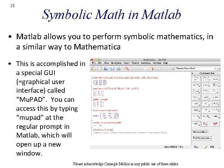
18 Symbolic Math in Matlab • Matlab allows you to perform symbolic mathematics, in a similar way to Mathematica • This is accomplished in a special GUI (=graphical user interface) called “Mu. PAD”. You can access this by typing “mupad” at the regular prompt in Matlab, which will open up a new window. Please acknowledge Carnegie Mellon in any public use of these slides

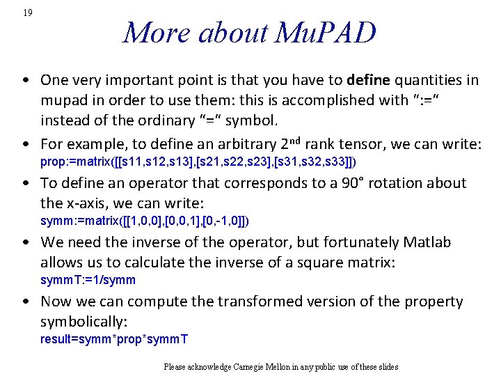
19 More about Mu. PAD • One very important point is that you have to define quantities in mupad in order to use them: this is accomplished with “: =“ instead of the ordinary “=“ symbol. • For example, to define an arbitrary 2 nd rank tensor, we can write: prop: =matrix([[s 11, s 12, s 13], [s 21, s 22, s 23], [s 31, s 32, s 33]]) • To define an operator that corresponds to a 90° rotation about the x-axis, we can write: symm: =matrix([[1, 0, 0], [0, 0, 1], [0, -1, 0]]) • We need the inverse of the operator, but fortunately Matlab allows us to calculate the inverse of a square matrix: symm. T: =1/symm • Now we can compute the transformed version of the property symbolically: result=symm*prop*symm. T Please acknowledge Carnegie Mellon in any public use of these slides

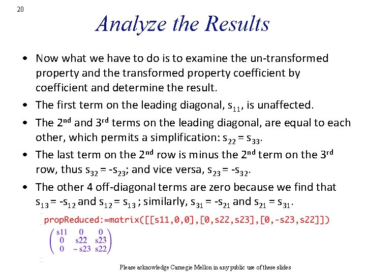
20 Analyze the Results • Now what we have to do is to examine the un-transformed property and the transformed property coefficient by coefficient and determine the result. • The first term on the leading diagonal, s 11, is unaffected. • The 2 nd and 3 rd terms on the leading diagonal, are equal to each other, which permits a simplification: s 22 = s 33. • The last term on the 2 nd row is minus the 2 nd term on the 3 rd row, thus s 32 = -s 23; and vice versa, s 23 = -s 32. • The other 4 off-diagonal terms are zero because we find that s 13 = -s 12 and s 12 = s 13 ; similarly, s 31 = -s 21 and s 21 = s 31. Please acknowledge Carnegie Mellon in any public use of these slides

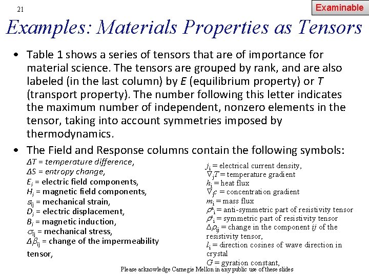
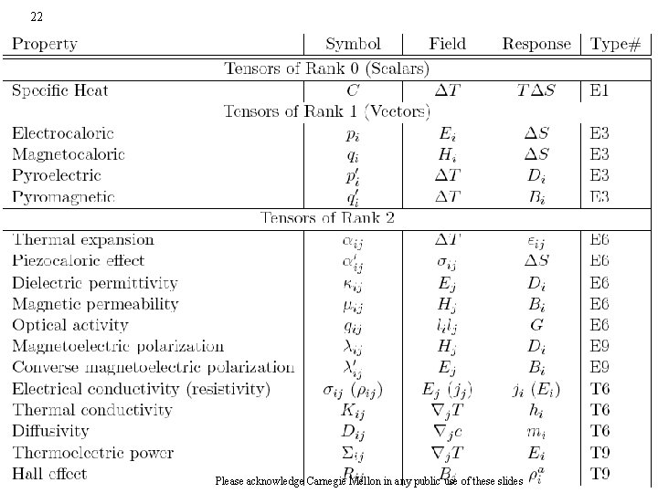
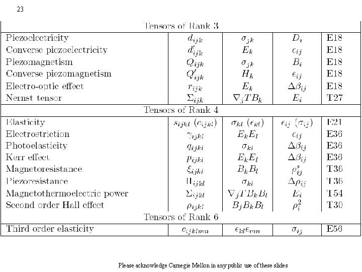
Examinable 21 Examples: Materials Properties as Tensors • Table 1 shows a series of tensors that are of importance for material science. The tensors are grouped by rank, and are also labeled (in the last column) by E (equilibrium property) or T (transport property). The number following this letter indicates the maximum number of independent, nonzero elements in the tensor, taking into account symmetries imposed by thermodynamics. • The Field and Response columns contain the following symbols: ∆T = temperature difference, ∆S = entropy change, Ei = electric field components, Hi = magnetic field components, ij = mechanical strain, Di = electric displacement, Bi = magnetic induction, ij = mechanical stress, ∆bij = change of the impermeability tensor, ji = electrical current density, j. T = temperature gradient hi = heat flux jc = concentration gradient mi = mass flux rai = anti-symmetric part of resistivity tensor rsi = symmetric part of resistivity tensor ∆rij = change in the component ij of the resistivity tensor, li = direction cosines of wave direction in crystal G = gyration constant, Please acknowledge Carnegie Mellon in any public use of these slides

22 Please acknowledge Carnegie Mellon in any public use of these slides

23 Please acknowledge Carnegie Mellon in any public use of these slides

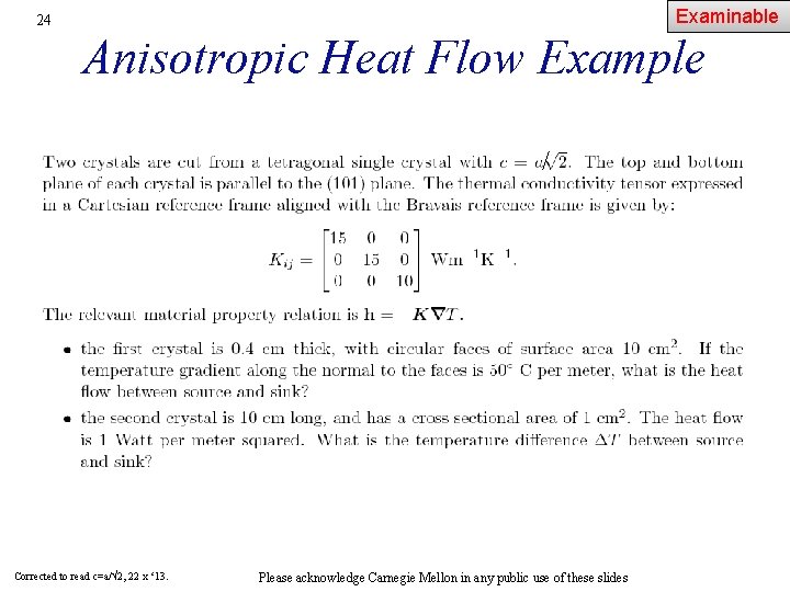
Examinable 24 Anisotropic Heat Flow Example / Corrected to read c=a/√ 2, 22 x ‘ 13. Please acknowledge Carnegie Mellon in any public use of these slides

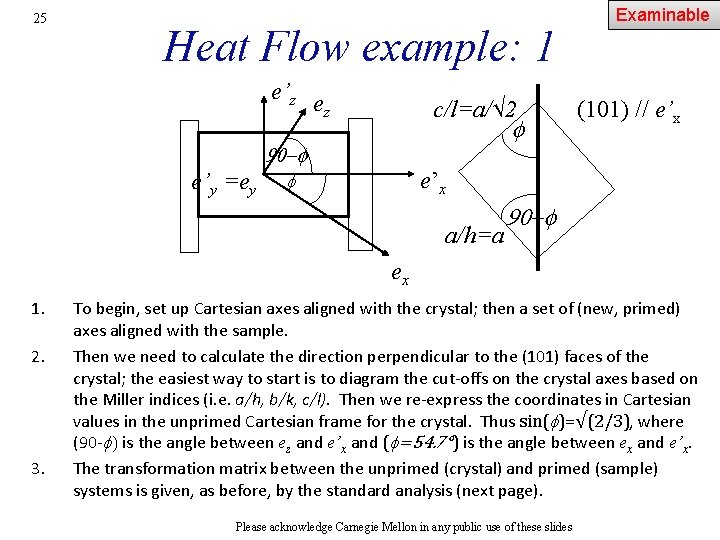
25 Heat Flow example: 1 e’z e z c/l=a/√ 2 f 90 -f e’y =ey Examinable (101) // e’x f a/h=a 90 -f ex 1. 2. 3. To begin, set up Cartesian axes aligned with the crystal; then a set of (new, primed) axes aligned with the sample. Then we need to calculate the direction perpendicular to the (101) faces of the crystal; the easiest way to start is to diagram the cut-offs on the crystal axes based on the Miller indices (i. e. a/h, b/k, c/l). Then we re-express the coordinates in Cartesian values in the unprimed Cartesian frame for the crystal. Thus sin(f)=√(2/3), where (90 -f) is the angle between ez and e’x and (f=54. 7°) is the angle between ex and e’x. The transformation matrix between the unprimed (crystal) and primed (sample) systems is given, as before, by the standard analysis (next page). Please acknowledge Carnegie Mellon in any public use of these slides

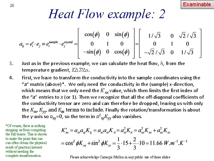
26 3. 4. Heat Flow example: 2 Examinable Just as in the previous example, we can calculate the heat flow, h, from the temperature gradient, K∆T/∆x. First, we have to transform the conductivity into the sample coordinates using the “a” matrix (above)*. We only need the conductivity in the (sample) x-direction, which means that we only need the K’xx value, which then limits the first index of the “a” entries to x (or 1). Then we recognize that all the off-diagonal coefficients of the conductivity tensor are zero and can therefore be dropped, leaving us with only the Kxx, Kyy, and Kzz terms to include. Finally the rotation/transformation is about the y-axis so axy=0, so the term in a 2 xy. Kyy also vanishes. *Of course, there is nothing stopping us from computing the full tensor. This is shown to make the point that one can often obtain the physical result of practical interest without needing the complete transformation. Please acknowledge Carnegie Mellon in any public use of these slides

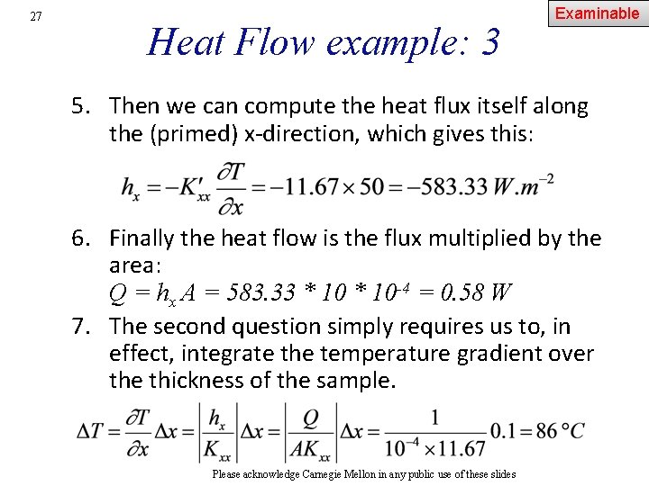
27 Heat Flow example: 3 Examinable 5. Then we can compute the heat flux itself along the (primed) x-direction, which gives this: 6. Finally the heat flow is the flux multiplied by the area: Q = hx A = 583. 33 * 10 -4 = 0. 58 W 7. The second question simply requires us to, in effect, integrate the temperature gradient over the thickness of the sample. Please acknowledge Carnegie Mellon in any public use of these slides

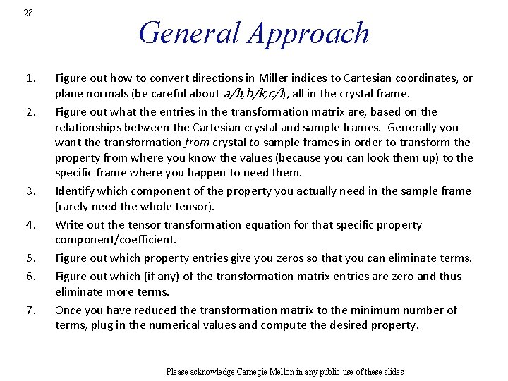
28 1. 2. 3. 4. 5. 6. 7. General Approach Figure out how to convert directions in Miller indices to Cartesian coordinates, or plane normals (be careful about a/h, b/k, c/l), all in the crystal frame. Figure out what the entries in the transformation matrix are, based on the relationships between the Cartesian crystal and sample frames. Generally you want the transformation from crystal to sample frames in order to transform the property from where you know the values (because you can look them up) to the specific frame where you happen to need them. Identify which component of the property you actually need in the sample frame (rarely need the whole tensor). Write out the tensor transformation equation for that specific property component/coefficient. Figure out which property entries give you zeros so that you can eliminate terms. Figure out which (if any) of the transformation matrix entries are zero and thus eliminate more terms. Once you have reduced the transformation matrix to the minimum number of terms, plug in the numerical values and compute the desired property. Please acknowledge Carnegie Mellon in any public use of these slides

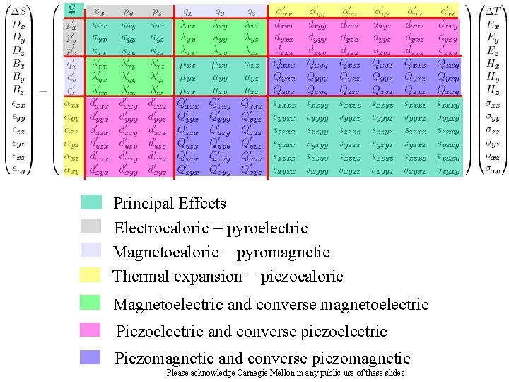
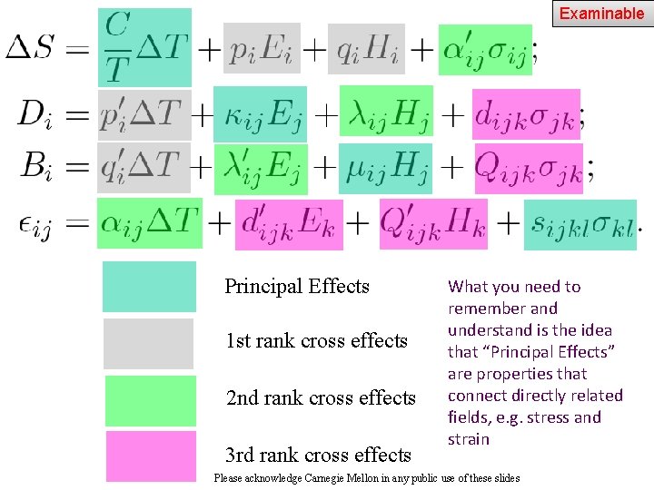
29 Principal Effects Electrocaloric = pyroelectric Magnetocaloric = pyromagnetic Thermal expansion = piezocaloric Magnetoelectric and converse magnetoelectric Piezoelectric and converse piezoelectric Piezomagnetic and converse piezomagnetic Please acknowledge Carnegie Mellon in any public use of these slides

Examinable 30 Principal Effects 1 st rank cross effects 2 nd rank cross effects 3 rd rank cross effects What you need to remember and understand is the idea that “Principal Effects” are properties that connect directly related fields, e. g. stress and strain Please acknowledge Carnegie Mellon in any public use of these slides

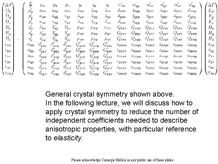
31 General crystal symmetry shown above. In the following lecture, we will discuss how to apply crystal symmetry to reduce the number of independent coefficients needed to describe anisotropic properties, with particular reference to elasticity. Please acknowledge Carnegie Mellon in any public use of these slides

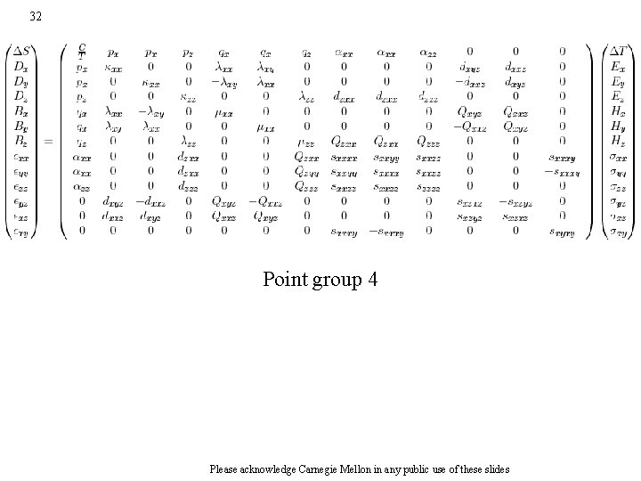
32 Point group 4 Please acknowledge Carnegie Mellon in any public use of these slides

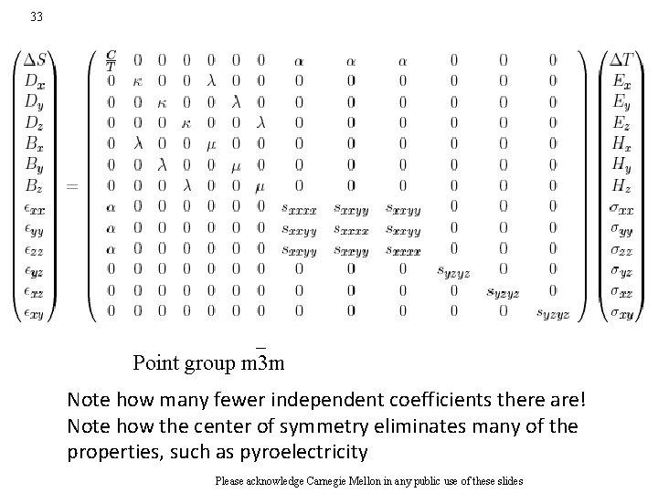
33 Point group m 3 m Note how many fewer independent coefficients there are! Note how the center of symmetry eliminates many of the properties, such as pyroelectricity Please acknowledge Carnegie Mellon in any public use of these slides

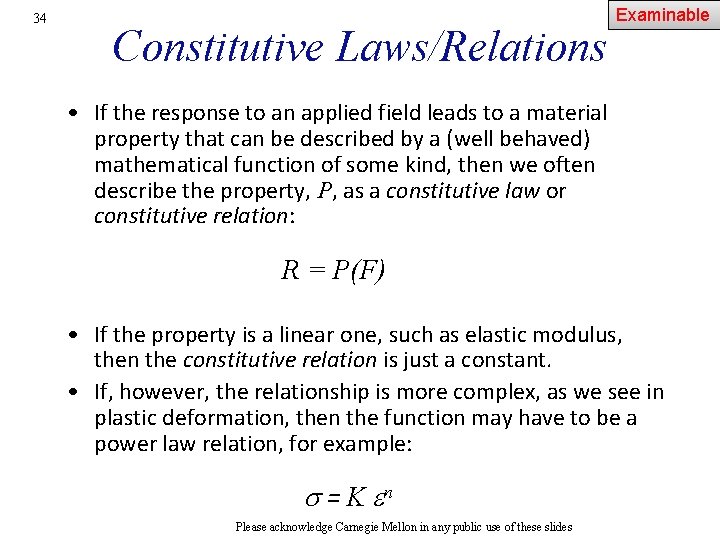
34 Constitutive Laws/Relations Examinable • If the response to an applied field leads to a material property that can be described by a (well behaved) mathematical function of some kind, then we often describe the property, P, as a constitutive law or constitutive relation: R = P(F) • If the property is a linear one, such as elastic modulus, then the constitutive relation is just a constant. • If, however, the relationship is more complex, as we see in plastic deformation, then the function may have to be a power law relation, for example: = K n Please acknowledge Carnegie Mellon in any public use of these slides

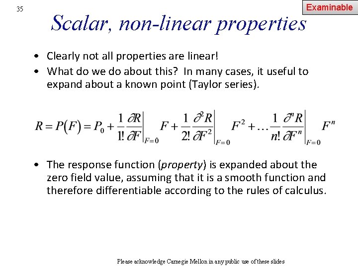
35 Examinable Scalar, non-linear properties • Clearly not all properties are linear! • What do we do about this? In many cases, it useful to expand about a known point (Taylor series). • The response function (property) is expanded about the zero field value, assuming that it is a smooth function and therefore differentiable according to the rules of calculus. Please acknowledge Carnegie Mellon in any public use of these slides

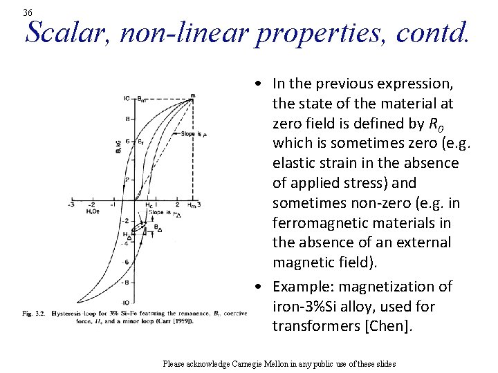
36 Scalar, non-linear properties, contd. • In the previous expression, the state of the material at zero field is defined by R 0 which is sometimes zero (e. g. elastic strain in the absence of applied stress) and sometimes non-zero (e. g. in ferromagnetic materials in the absence of an external magnetic field). • Example: magnetization of iron-3%Si alloy, used for transformers [Chen]. Please acknowledge Carnegie Mellon in any public use of these slides

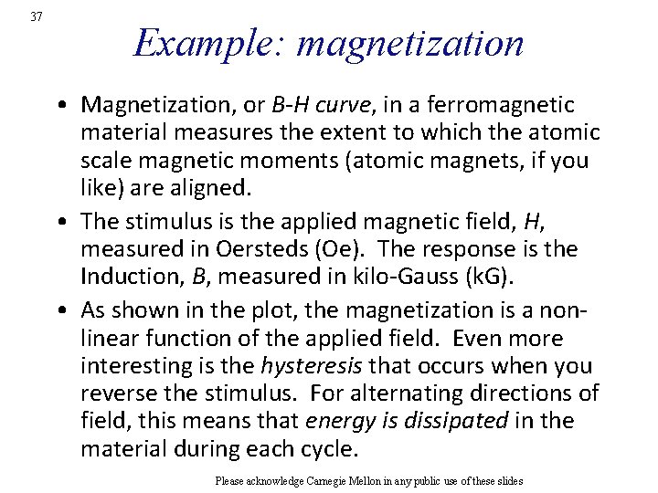
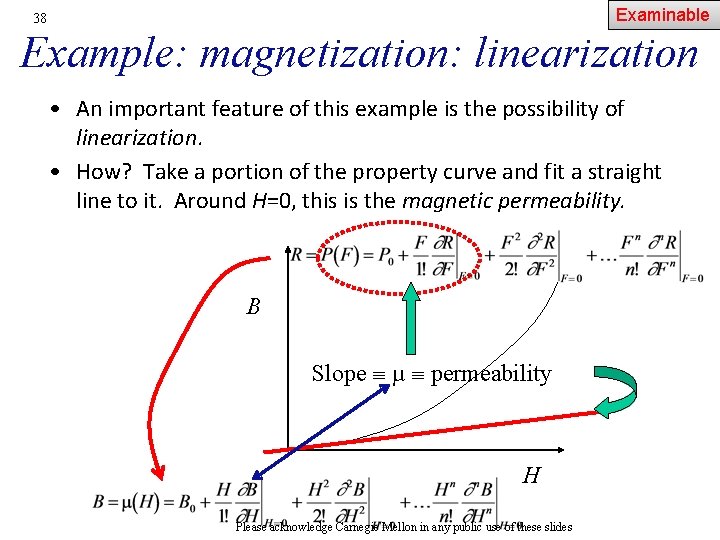
37 Example: magnetization • Magnetization, or B-H curve, in a ferromagnetic material measures the extent to which the atomic scale magnetic moments (atomic magnets, if you like) are aligned. • The stimulus is the applied magnetic field, H, measured in Oersteds (Oe). The response is the Induction, B, measured in kilo-Gauss (k. G). • As shown in the plot, the magnetization is a nonlinear function of the applied field. Even more interesting is the hysteresis that occurs when you reverse the stimulus. For alternating directions of field, this means that energy is dissipated in the material during each cycle. Please acknowledge Carnegie Mellon in any public use of these slides

Examinable 38 Example: magnetization: linearization • An important feature of this example is the possibility of linearization. • How? Take a portion of the property curve and fit a straight line to it. Around H=0, this is the magnetic permeability. B Slope µ permeability H Please acknowledge Carnegie Mellon in any public use of these slides

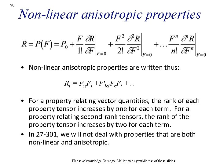
39 Non-linear anisotropic properties • Non-linear anisotropic properties are written thus: Ri = Pij. Fj +P'ikl. Fk. Fl +… • For a property relating vector quantities, the rank of each property tensor increases by one for each term. For a property relating second-rank tensors, the rank of the property tensor increases by two for each term. • In 27 -301, we will not deal with properties that are both non-linear and anisotropic. Please acknowledge Carnegie Mellon in any public use of these slides

40 Summary • Crystal symmetry limits the number of independent coefficients in a property tensor. • The method that we use to reduce the number of coefficients is by noting that, if we apply crystal symmetry, we cannot tell that anything is different about the crystal. This means that the properties of the crystal must be unchanged. This in turn means that each entry in the property tensor must be the same. • Therefore we can equate the property tensor before and after application of a symmetry element. • Lists of anisotropic properties are given. • An example is given of how the list of coefficients is reduced, sometimes drastically, by crystal symmetry. • Non-linear effects are briefly mentioned. Please acknowledge Carnegie Mellon in any public use of these slides

41 Supplemental Slides Please acknowledge Carnegie Mellon in any public use of these slides

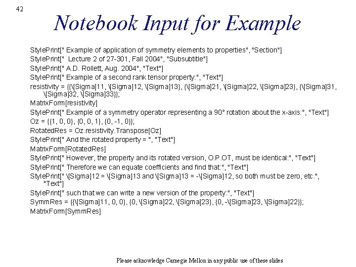
42 Notebook Input for Example Style. Print[" Example of application of symmetry elements to properties", "Section"] Style. Print[" Lecture 2 of 27 -301, Fall 2004", "Subsubtitle"] Style. Print[" A. D. Rollett, Aug. 2004", "Text"] Style. Print[" Example of a second rank tensor property: ", "Text"] resistivity = {{[Sigma]11, [Sigma]12, [Sigma]13}, {[Sigma]21, [Sigma]22, [Sigma]23}, {[Sigma]31, [Sigma]32, [Sigma]33}}; Matrix. Form[resistivity] Style. Print[" Example of a symmetry operator representing a 90° rotation about the x-axis: ", "Text"] Oz = {{1, 0, 0}, {0, 0, 1}, {0, -1, 0}}; Rotated. Res = Oz. resistivity. Transpose[Oz] Style. Print[" And the rotated property = ", "Text"] Matrix. Form[Rotated. Res] Style. Print[" However, the property and its rotated version, O. P. OT, must be identical: ", "Text"] Style. Print[" Therefore we can equate coefficients and find that: ", "Text"] Style. Print[" [Sigma]12 = [Sigma]13 and [Sigma]13 = -[Sigma]12, so both must be zero, etc. ", "Text"] Style. Print[" such that we can write a new version of the property: ", "Text"] Symm. Res = {{[Sigma]11, 0, 0}, {0, [Sigma]22, [Sigma]23}, {0, -[Sigma]23, [Sigma]22}}; Matrix. Form[Symm. Res] Please acknowledge Carnegie Mellon in any public use of these slides

43 Examinable Please acknowledge Carnegie Mellon in any public use of these slides

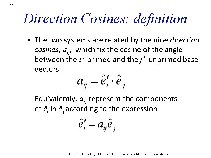
44 Direction Cosines: definition • The two systems are related by the nine direction cosines, aij, which fix the cosine of the angle between the ith primed and the jth unprimed base vectors: Equivalently, aij represent the components of êi in êj according to the expression Please acknowledge Carnegie Mellon in any public use of these slides

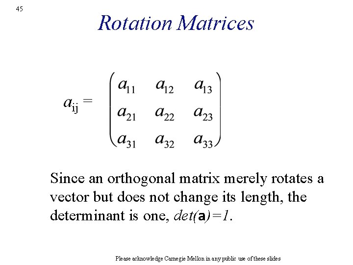
45 Rotation Matrices aij = Since an orthogonal matrix merely rotates a vector but does not change its length, the determinant is one, det(a)=1. Please acknowledge Carnegie Mellon in any public use of these slides

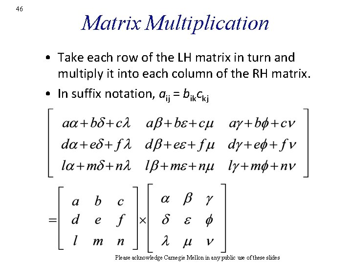
46 Matrix Multiplication • Take each row of the LH matrix in turn and multiply it into each column of the RH matrix. • In suffix notation, aij = bikckj Please acknowledge Carnegie Mellon in any public use of these slides

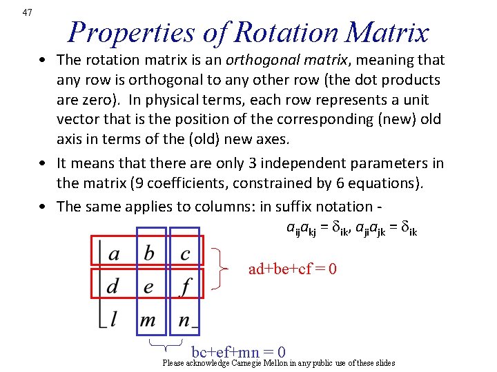
47 Properties of Rotation Matrix • The rotation matrix is an orthogonal matrix, meaning that any row is orthogonal to any other row (the dot products are zero). In physical terms, each row represents a unit vector that is the position of the corresponding (new) old axis in terms of the (old) new axes. • It means that there are only 3 independent parameters in the matrix (9 coefficients, constrained by 6 equations). • The same applies to columns: in suffix notation aijakj = dik, ajiajk = dik ad+be+cf = 0 bc+ef+mn = 0 Please acknowledge Carnegie Mellon in any public use of these slides

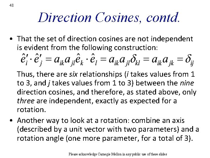
48 Direction Cosines, contd. • That the set of direction cosines are not independent is evident from the following construction: Thus, there are six relationships (i takes values from 1 to 3, and j takes values from 1 to 3) between the nine direction cosines, and therefore, as stated above, only three are independent, exactly as expected for a rotation. • Another way to look at a rotation: combine an axis (described by a unit vector with two parameters) and a rotation angle (one more parameter, for a total of 3). Please acknowledge Carnegie Mellon in any public use of these slides

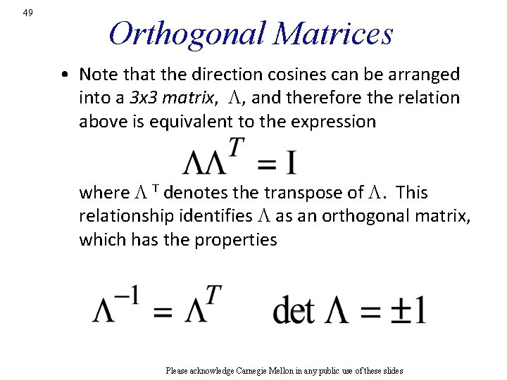
49 Orthogonal Matrices • Note that the direction cosines can be arranged into a 3 x 3 matrix, L, and therefore the relation above is equivalent to the expression where L T denotes the transpose of L. This relationship identifies L as an orthogonal matrix, which has the properties Please acknowledge Carnegie Mellon in any public use of these slides

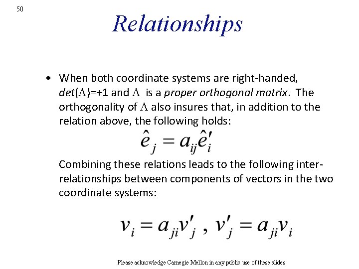
50 Relationships • When both coordinate systems are right-handed, det(L)=+1 and L is a proper orthogonal matrix. The orthogonality of L also insures that, in addition to the relation above, the following holds: Combining these relations leads to the following interrelationships between components of vectors in the two coordinate systems: Please acknowledge Carnegie Mellon in any public use of these slides

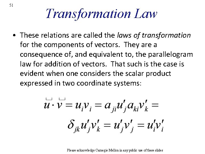
51 Transformation Law • These relations are called the laws of transformation for the components of vectors. They are a consequence of, and equivalent to, the parallelogram law for addition of vectors. That such is the case is evident when one considers the scalar product expressed in two coordinate systems: Please acknowledge Carnegie Mellon in any public use of these slides

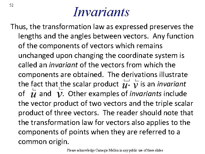
52 Invariants Thus, the transformation law as expressed preserves the lengths and the angles between vectors. Any function of the components of vectors which remains unchanged upon changing the coordinate system is called an invariant of the vectors from which the components are obtained. The derivations illustrate the fact that the scalar product is an invariant of and. Other examples of invariants include the vector product of two vectors and the triple scalar product of three vectors. The reader should note that the transformation law for vectors also applies to the components of points when they are referred to a common origin. Please acknowledge Carnegie Mellon in any public use of these slides

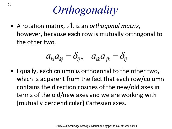
53 Orthogonality • A rotation matrix, L, is an orthogonal matrix, however, because each row is mutually orthogonal to the other two. • Equally, each column is orthogonal to the other two, which is apparent from the fact that each row/column contains the direction cosines of the new/old axes in terms of the old/new axes and we are working with [mutually perpendicular] Cartesian axes. Please acknowledge Carnegie Mellon in any public use of these slides