1 27 301 MicrostructureProperties Tensors and Anisotropy Part

1 27 -301 Microstructure-Properties Tensors and Anisotropy, Part 1 Profs. A. D. Rollett, M. De Graef Processing Performance Microstructure Properties Last modified: 4 th Oct. ‘ 15 Please acknowledge Carnegie Mellon if you make public use of these slides

2 Objective • The objective of this lecture is to explain the meaning of analytical material properties and how to describe their anisotropy. • Tensors are defined and explained, along with the Tensor Transformation Rule. • We use tensors to describe both fields (stimuli and responses) and properties. Accordingly we describe their properties and how to work examples of anisotropic properties, including the effect of crystal symmetry. • A central topic is that of the effect of rotations, expressed as axis transformations (this lecture) and symmetry operators (next lecture). • All properties described in this section are linear properties. Please acknowledge Carnegie Mellon if you make public use of these slides

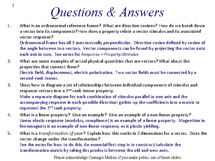
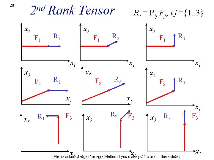
3 1. 2. 3. 4. 5. Questions & Answers What is an orthonormal reference frame? What are direction cosines? How do we break down a vector into its components? How does a property relate a vector stimulus and its associated vector response? Orthonormal frame has all 3 axes mutually perpendicular. Direction cosine defined by cosine of the angle between two vectors. Vector components can be found by projecting the vector onto each axis in turn. See notes for Response = Property: Stimulus What are some examples of actual physical quantities that are vectors? What about the properties that connect them? Electric field, displacement, electric polarization. Two vector fields must be connected by a second-rank tensor. Show to diagram a set of relationships between individual components of stimulus and response vectors into a 2 nd rank tensor property. Make a separate diagram for each combination of stimulus parallel to one axis and the accompanying response in each possible direction; gather up the coefficients into a matrix to represent the 2 nd rank property. What is a linear property? Give an example of a non-linear property? Linear elastic response (modulus, compliance) is an example of a linear property. Magnetism in ferromagnets is an example of non-linear response, as is plastic yielding. What is a transformation of axes? Explain how this works in 2 dimensions for a vector. Does the vector change under the transformation? See the notes for how to do this. An essential first step is to construct/calculate the transformation matrix by taking dot products between the old and new axes. Please acknowledge Carnegie Mellon if you make public use of these slides

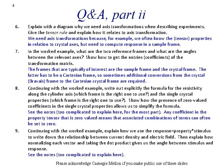
4 Q&A, part ii 6. 7. 8. 9. Explain with a diagram why we need axis transformations when describing experiments. Give the tensor rule and explain how it relates to axis transformation. We need axis transformations because, for example, we often know the (tensor) properties in relation to crystal axes, but need to compute response in a sample frame. In the worked example, what are the two reference frames and what are the angles between the relevant axes? Show to get the entries (coefficients) of the transformation matrix. The frames that are typically of interest are the sample frame and the crystal frame. The latter has to be a Cartesian frame, so sometimes additional conversions from the crystal (Bravais) frame to the Cartesian crystal frame are required. Continuing with the worked example, write out explicitly the formula for the resistivity along the cylinder axis (which frame is the right one to use? ) and the single crystal properties (which frame is the right one to use? ). Show the presence of zero-valued coefficients in the single crystal properties allows us to simplify the formula. See the notes (too complicated to explain here, for the most part). Any coefficient in the property tensor that is zero valued means that associated combinations of terms can often be set to zero. Continuing with the worked example, explain how we use the response=property*stimulus to write down the relationship between current density and electric field. Then explain how normalizing each vector and taking the dot product gives us the angle between stimulus and response. See the notes (too complicated to explain here). Please acknowledge Carnegie Mellon if you make public use of these slides

5 Q&A, part iii 10. What is the Einstein convention? The Einstein convention is that repeated indices (generally on the RHS) are implied sums. That is, wherever you see a repeated index, assume that you should sum up all terms involving that index over the range of (integer) values that apply (usually 1, 2 and 3). If you see an index in parentheses that is repeated, it is generally not subject to the convention. Please acknowledge Carnegie Mellon if you make public use of these slides

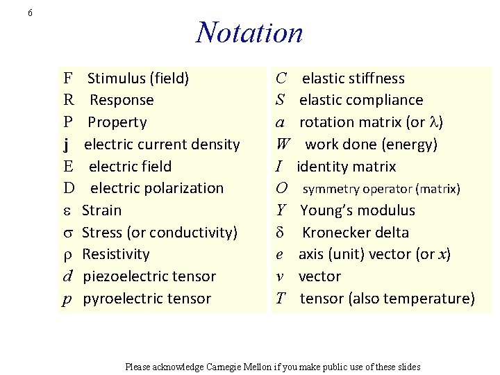
6 Notation F R P j E D e s r d p Stimulus (field) Response Property electric current density electric field electric polarization Strain Stress (or conductivity) Resistivity piezoelectric tensor pyroelectric tensor C S a W I O Y d e v T elastic stiffness elastic compliance rotation matrix (or l) work done (energy) identity matrix symmetry operator (matrix) Young’s modulus Kronecker delta axis (unit) vector (or x) vector tensor (also temperature) Please acknowledge Carnegie Mellon if you make public use of these slides

7 Mathematical Descriptions • [From L 1] Some properties have rigorous physical definitions, with well defined values, such as elastic modulus, thermal conductivity. There is a straightforward physical basis for the property and they can be predicted based on a knowledge of the component atoms and atomic structure. Nevertheless, most such properties are sensitive to microstructure. We discuss in this lecture these “Analytical Properties” since we can use analytical expressions of the type: Response = Property Stimulus e. g. , Stress = Modulus Strain • Mathematical descriptions of analytical properties are straightforward because of their linear nature. • Mathematics, tensor mathematics in particular, provides a quantitative framework. It is always necessary, however, to make a correspondence between mathematical variables and physical quantities. • In group theory one might say that there is a set of mathematical operations & parameters, and a set of physical quantities and processes: if the mathematics is a good description, then the two sets are isomorphous. Please acknowledge Carnegie Mellon if you make public use of these slides

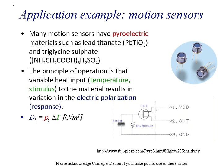
8 Application example: motion sensors • Many motion sensors have pyroelectric materials such as lead titanate (Pb. Ti. O 3) and triglycine sulphate ((NH 2 COOH)3 H 2 SO 4). • The principle of operation is that variable heat input (temperature, stimulus) to the material results in variation in the electric polarization (response). • Di = pi ∆T [C/m 2] http: //www. fuji-piezo. com/Pyro 3. htm#High%20 Sensitivity Please acknowledge Carnegie Mellon if you make public use of these slides

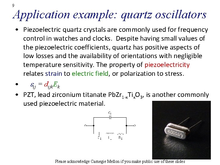
9 Application example: quartz oscillators • Piezoelectric quartz crystals are commonly used for frequency control in watches and clocks. Despite having small values of the piezoelectric coefficients, quartz has positive aspects of low losses and the availability of orientations with negligible temperature sensitivity. The property of piezoelectricity relates strain to electric field, or polarization to stress. • ij = dijk. Ek • PZT, lead zirconium titanate Pb. Zr 1 -x. Tix. O 3, is another commonly used piezoelectric material. Please acknowledge Carnegie Mellon if you make public use of these slides

10 Topics • Response = Property x Stimulus • Linear Properties • Axis transformations (changing the coordinate system) • Scalars, vectors and tensors • Tensor Transformation Rule • 1 st Example Please acknowledge Carnegie Mellon if you make public use of these slides

11 Math of Microstructure-Property Relationships • In order to describe properties, we must first relate a response to a stimulus with a property. • A stimulus is something that one does to a material, e. g. apply a load. • A response is something that is the result of applying a stimulus, e. g. if you apply a load (stress), the material will change shape (strain). • The material property is the connection between the stimulus and the response. Please acknowledge Carnegie Mellon if you make public use of these slides

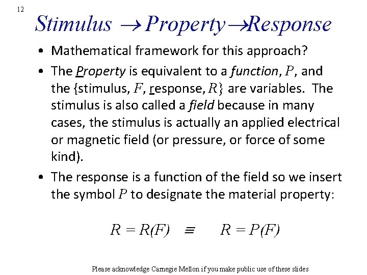
12 Stimulus Property Response • Mathematical framework for this approach? • The Property is equivalent to a function, P, and the {stimulus, F, response, R} are variables. The stimulus is also called a field because in many cases, the stimulus is actually an applied electrical or magnetic field (or pressure, or force of some kind). • The response is a function of the field so we insert the symbol P to designate the material property: R = R(F) R = P(F) Please acknowledge Carnegie Mellon if you make public use of these slides

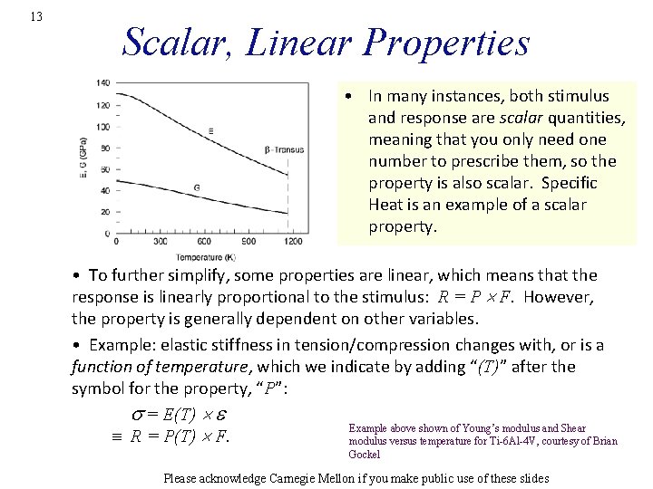
13 Scalar, Linear Properties • In many instances, both stimulus and response are scalar quantities, meaning that you only need one number to prescribe them, so the property is also scalar. Specific Heat is an example of a scalar property. • To further simplify, some properties are linear, which means that the response is linearly proportional to the stimulus: R = P F. However, the property is generally dependent on other variables. • Example: elastic stiffness in tension/compression changes with, or is a function of temperature, which we indicate by adding “(T)” after the symbol for the property, “P”: s = E(T) Example above shown of Young’s modulus and Shear R = P(T) F. modulus versus temperature for Ti-6 Al-4 V, courtesy of Brian Gockel Please acknowledge Carnegie Mellon if you make public use of these slides

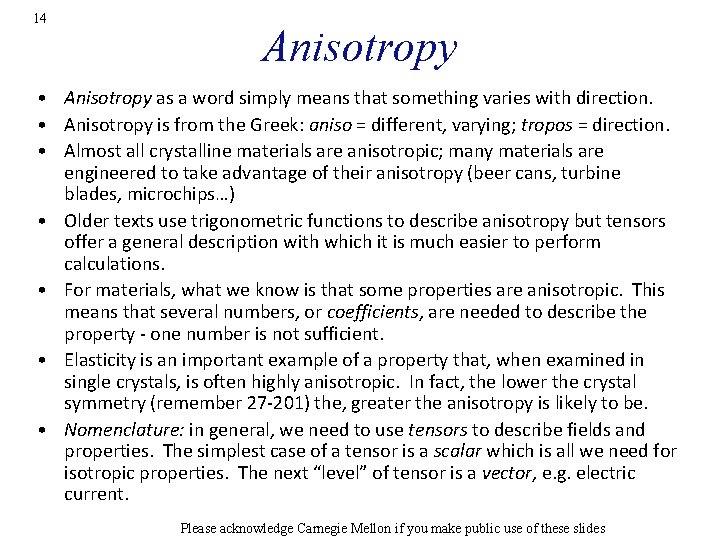
14 Anisotropy • Anisotropy as a word simply means that something varies with direction. • Anisotropy is from the Greek: aniso = different, varying; tropos = direction. • Almost all crystalline materials are anisotropic; many materials are engineered to take advantage of their anisotropy (beer cans, turbine blades, microchips…) • Older texts use trigonometric functions to describe anisotropy but tensors offer a general description with which it is much easier to perform calculations. • For materials, what we know is that some properties are anisotropic. This means that several numbers, or coefficients, are needed to describe the property - one number is not sufficient. • Elasticity is an important example of a property that, when examined in single crystals, is often highly anisotropic. In fact, the lower the crystal symmetry (remember 27 -201) the, greater the anisotropy is likely to be. • Nomenclature: in general, we need to use tensors to describe fields and properties. The simplest case of a tensor is a scalar which is all we need for isotropic properties. The next “level” of tensor is a vector, e. g. electric current. Please acknowledge Carnegie Mellon if you make public use of these slides

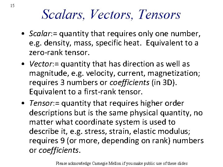
15 Scalars, Vectors, Tensors • Scalar: = quantity that requires only one number, e. g. density, mass, specific heat. Equivalent to a zero-rank tensor. • Vector: = quantity that has direction as well as magnitude, e. g. velocity, current, magnetization; requires 3 numbers or coefficients (in 3 D). Equivalent to a first-rank tensor. • Tensor: = quantity that requires higher order descriptions but is the same physical quantity, no matter what coordinate system is used to describe it, e. g. stress, strain, elastic modulus; requires 9 (or more, depending on rank) numbers or coefficients. Please acknowledge Carnegie Mellon if you make public use of these slides

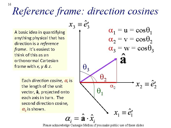
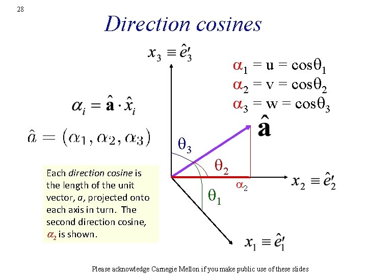
16 Reference frame: direction cosines A basic idea in quantifying anything physical that has direction is a reference frame. It’s easiest to think of this as an orthonormal Cartesian frame with x, y & z. Each direction cosine, a, is the length of the unit vector, â, projected onto each axis in turn. The second direction cosine, a 2 is shown. a 1 = u = cosq 1 a 2 = v = cosq 2 a 3 = w = cosq 3 q 2 q 1 a 2 Please acknowledge Carnegie Mellon if you make public use of these slides

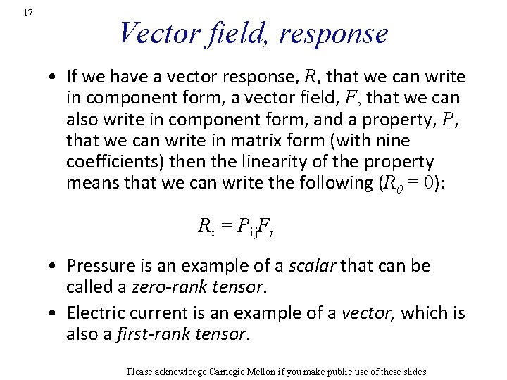
17 Vector field, response • If we have a vector response, R, that we can write in component form, a vector field, F, that we can also write in component form, and a property, P, that we can write in matrix form (with nine coefficients) then the linearity of the property means that we can write the following (R 0 = 0): Ri = Pij. Fj • Pressure is an example of a scalar that can be called a zero-rank tensor. • Electric current is an example of a vector, which is also a first-rank tensor. Please acknowledge Carnegie Mellon if you make public use of these slides

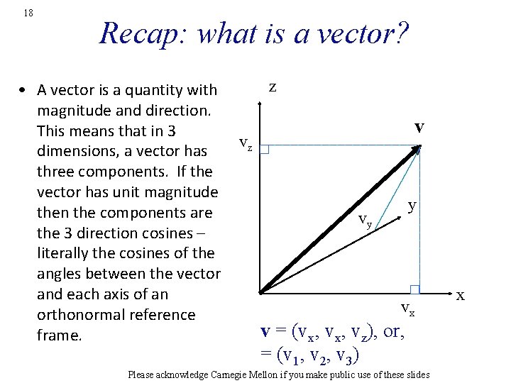
18 Recap: what is a vector? • A vector is a quantity with magnitude and direction. This means that in 3 dimensions, a vector has three components. If the vector has unit magnitude then the components are the 3 direction cosines – literally the cosines of the angles between the vector and each axis of an orthonormal reference frame. z v vz y vy vx v = (vx, vz), or, = (v 1, v 2, v 3) Please acknowledge Carnegie Mellon if you make public use of these slides x

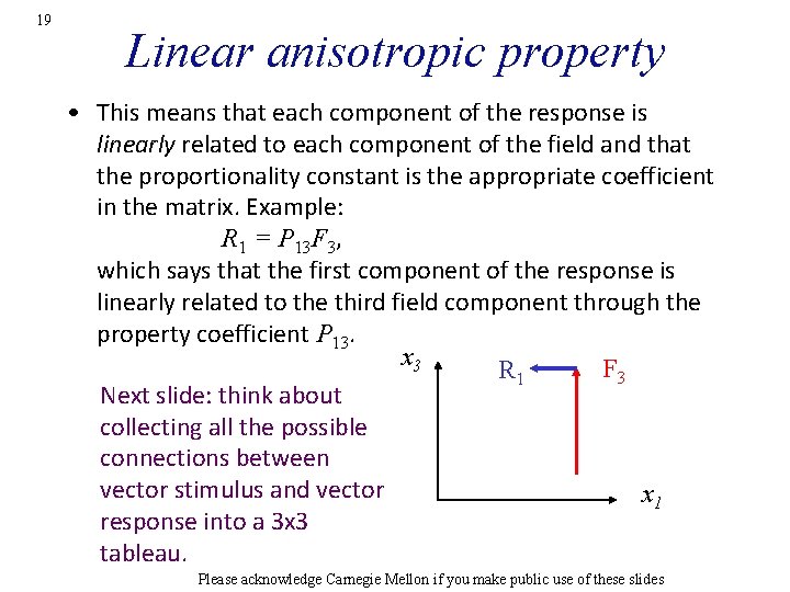
19 Linear anisotropic property • This means that each component of the response is linearly related to each component of the field and that the proportionality constant is the appropriate coefficient in the matrix. Example: R 1 = P 13 F 3, which says that the first component of the response is linearly related to the third field component through the property coefficient P 13. x 3 F 3 R 1 Next slide: think about collecting all the possible connections between vector stimulus and vector x 1 response into a 3 x 3 tableau. Please acknowledge Carnegie Mellon if you make public use of these slides

nd 2 Rank Tensor 20 x 3 F 1 x 3 R 1 F 2 F 2 x 3 F 3 R 3 x 1 x 3 R 2 F 2 R 3 x 1 R 1 F 1 x 3 R 2 x 1 x 3 Ri = Pij Fj, i, j ={1. . 3} x 3 R 2 F 3 x 3 R 3 x 1 public use of these slides x 1 Please acknowledge Carnegie Mellon if you make x 1 F 3 x 1

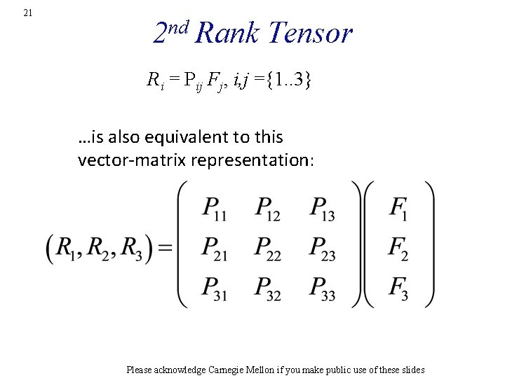
21 nd 2 Rank Tensor Ri = Pij Fj, i, j ={1. . 3} …is also equivalent to this vector-matrix representation: Please acknowledge Carnegie Mellon if you make public use of these slides

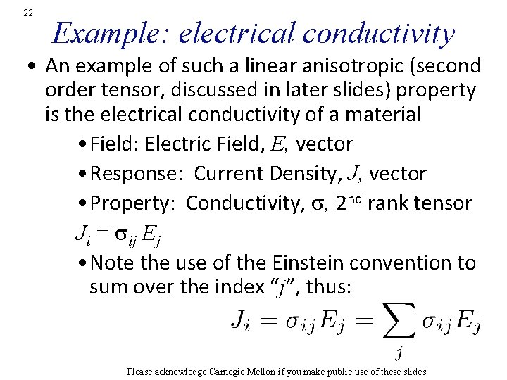
22 Example: electrical conductivity • An example of such a linear anisotropic (second order tensor, discussed in later slides) property is the electrical conductivity of a material • Field: Electric Field, E, vector • Response: Current Density, J, vector • Property: Conductivity, s, 2 nd rank tensor Ji = sij Ej • Note the use of the Einstein convention to sum over the index “j”, thus: Please acknowledge Carnegie Mellon if you make public use of these slides

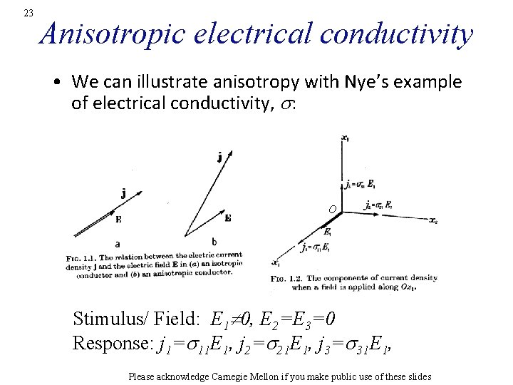
23 Anisotropic electrical conductivity • We can illustrate anisotropy with Nye’s example of electrical conductivity, s: O Stimulus/ Field: E 1 0, E 2=E 3=0 Response: j 1=s 11 E 1, j 2=s 21 E 1, j 3=s 31 E 1, Please acknowledge Carnegie Mellon if you make public use of these slides

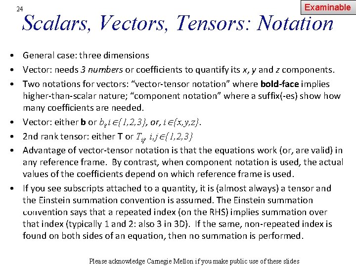
Examinable 24 Scalars, Vectors, Tensors: Notation • General case: three dimensions • Vector: needs 3 numbers or coefficients to quantify its x, y and z components. • Two notations for vectors: “vector-tensor notation” where bold-face implies higher-than-scalar nature; “component notation” where a suffix(-es) show many coefficients are needed. • Vector: either b or bi, i {1, 2, 3}, or, i {x, y, z}. • 2 nd rank tensor: either T or Tij, i, j {1, 2, 3} • Advantage of vector-tensor notation is that the equations work (or, are valid) in any reference frame. By contrast, when component notation is used, the actual values of the coefficients depend on which reference frame is used. • If you see subscripts attached to a quantity, it is (almost always) a tensor and the Einstein summation convention is assumed. The Einstein summation convention says that a repeated index (on the RHS) implies summation over that index (typically 1 and 2: also 3 in 3 D). If the same, non-repeated index is found on both sides of an equation, then no summation is performed. Please acknowledge Carnegie Mellon if you make public use of these slides

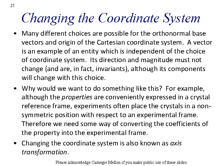
25 Changing the Coordinate System • Many different choices are possible for the orthonormal base vectors and origin of the Cartesian coordinate system. A vector is an example of an entity which is independent of the choice of coordinate system. Its direction and magnitude must not change (and are, in fact, invariants), although its components will change with this choice. • Why would we want to do something like this? For example, although the properties are conveniently expressed in a crystal reference frame, experiments often place the crystals in a nonsymmetric position with respect to an experimental frame. Therefore we need some way of converting the coefficients of the property into the experimental frame. • Changing the coordinate system is also known as axis transformation. Please acknowledge Carnegie Mellon if you make public use of these slides

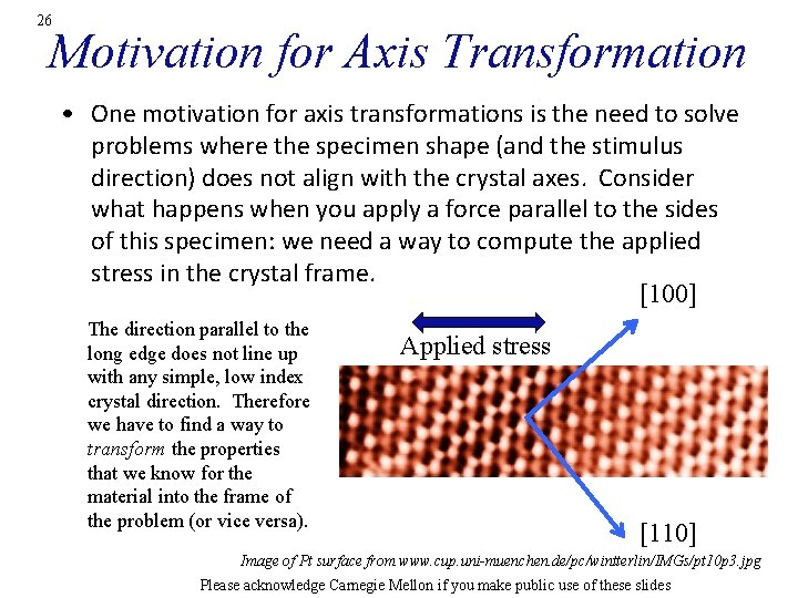
26 Motivation for Axis Transformation • One motivation for axis transformations is the need to solve problems where the specimen shape (and the stimulus direction) does not align with the crystal axes. Consider what happens when you apply a force parallel to the sides of this specimen: we need a way to compute the applied stress in the crystal frame. [100] The direction parallel to the long edge does not line up with any simple, low index crystal direction. Therefore we have to find a way to transform the properties that we know for the material into the frame of the problem (or vice versa). Applied stress [110] Image of Pt surface from www. cup. uni-muenchen. de/pc/wintterlin/IMGs/pt 10 p 3. jpg Please acknowledge Carnegie Mellon if you make public use of these slides

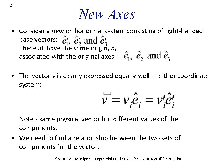
27 New Axes • Consider a new orthonormal system consisting of right-handed base vectors: These all have the same origin, o, associated with the original axes: • The vector v is clearly expressed equally well in either coordinate system: Note - same physical vector but different values of the components. • We need to find a relationship between the two sets of components for the vector. Please acknowledge Carnegie Mellon if you make public use of these slides

28 Direction cosines a 1 = u = cosq 1 a 2 = v = cosq 2 a 3 = w = cosq 3 Each direction cosine is the length of the unit vector, a, projected onto each axis in turn. The second direction cosine, a 2 is shown. q 2 q 1 a 2 Please acknowledge Carnegie Mellon if you make public use of these slides

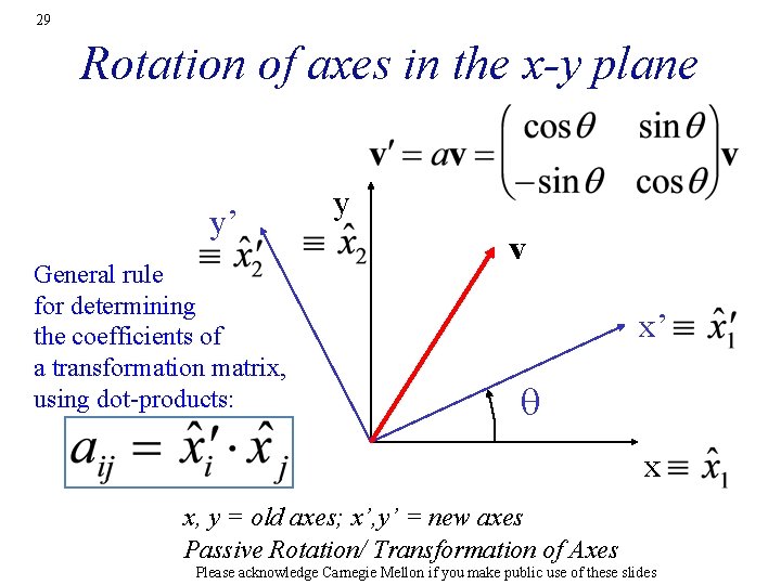
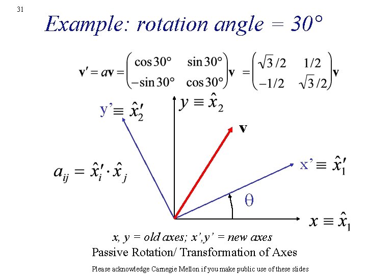
29 Rotation of axes in the x-y plane y’ General rule for determining the coefficients of a transformation matrix, using dot-products: y v x’ q x x, y = old axes; x’, y’ = new axes Passive Rotation/ Transformation of Axes Please acknowledge Carnegie Mellon if you make public use of these slides

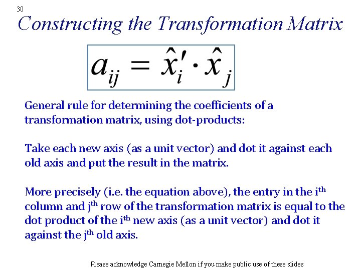
30 Constructing the Transformation Matrix General rule for determining the coefficients of a transformation matrix, using dot-products: Take each new axis (as a unit vector) and dot it against each old axis and put the result in the matrix. More precisely (i. e. the equation above), the entry in the i th column and jth row of the transformation matrix is equal to the dot product of the ith new axis (as a unit vector) and dot it against the jth old axis. Please acknowledge Carnegie Mellon if you make public use of these slides

31 Example: rotation angle = 30° y’ v x’ q x, y = old axes; x’, y’ = new axes Passive Rotation/ Transformation of Axes Please acknowledge Carnegie Mellon if you make public use of these slides

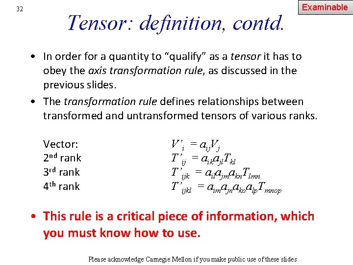
32 Tensor: definition, contd. Examinable • In order for a quantity to “qualify” as a tensor it has to obey the axis transformation rule, as discussed in the previous slides. • The transformation rule defines relationships between transformed and untransformed tensors of various ranks. Vector: 2 nd rank 3 rd rank 4 th rank V’i = aij. Vj T’ij = aikajl. Tkl T’ijk = ailajmakn. Tlmn T’ijkl = aimajnakoalp. Tmnop • This rule is a critical piece of information, which you must know how to use. Please acknowledge Carnegie Mellon if you make public use of these slides

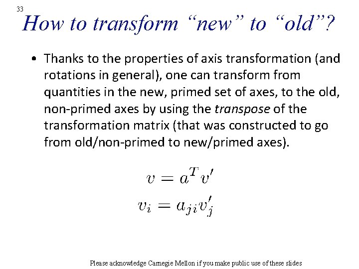
33 How to transform “new” to “old”? • Thanks to the properties of axis transformation (and rotations in general), one can transform from quantities in the new, primed set of axes, to the old, non-primed axes by using the transpose of the transformation matrix (that was constructed to go from old/non-primed to new/primed axes). Please acknowledge Carnegie Mellon if you make public use of these slides

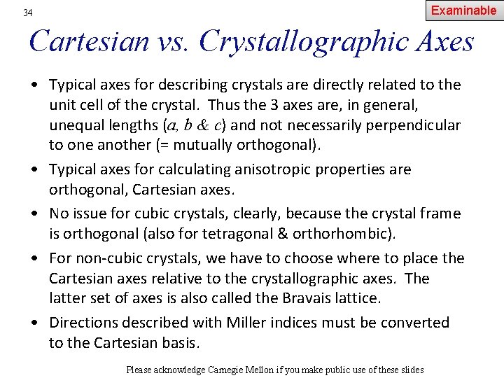
Examinable 34 Cartesian vs. Crystallographic Axes • Typical axes for describing crystals are directly related to the unit cell of the crystal. Thus the 3 axes are, in general, unequal lengths (a, b & c) and not necessarily perpendicular to one another (= mutually orthogonal). • Typical axes for calculating anisotropic properties are orthogonal, Cartesian axes. • No issue for cubic crystals, clearly, because the crystal frame is orthogonal (also for tetragonal & orthorhombic). • For non-cubic crystals, we have to choose where to place the Cartesian axes relative to the crystallographic axes. The latter set of axes is also called the Bravais lattice. • Directions described with Miller indices must be converted to the Cartesian basis. Please acknowledge Carnegie Mellon if you make public use of these slides

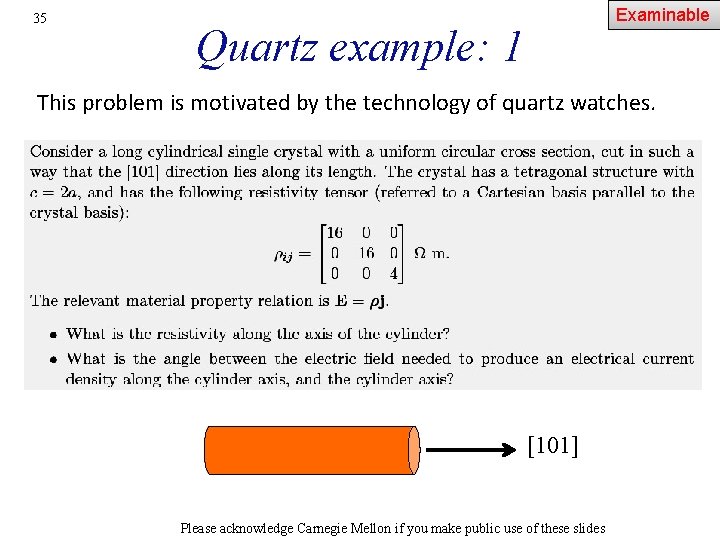
35 Examinable Quartz example: 1 This problem is motivated by the technology of quartz watches. [101] Please acknowledge Carnegie Mellon if you make public use of these slides

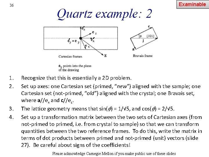
36 1. 2. 3. 4. Quartz example: 2 Examinable Recognize that this is essentially a 2 D problem. Set up axes: one Cartesian set (primed, “new”) aligned with the sample; one Cartesian set (not-primed, “old”) aligned with the crystal; one Bravais set, where a//ex and c//ez. The lattice geometry means that sin(f) = 1/√ 5, and cos(f) = 2/√ 5. Set up a transformation matrix between the two sets of Cartesian axes (from not-primed to primed, i. e. from crystal to sample) so that we can transform quantities between the two reference frames. To do this, write the matrix in terms of dot products between primed and not-primed (unit) vectors (slide 27). Be careful about signs of the coefficients! Please acknowledge Carnegie Mellon if you make public use of these slides

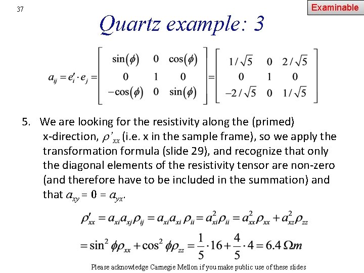
37 Quartz example: 3 Examinable 5. We are looking for the resistivity along the (primed) x-direction, r’xx (i. e. x in the sample frame), so we apply the transformation formula (slide 29), and recognize that only the diagonal elements of the resistivity tensor are non-zero (and therefore have to be included in the summation) and that axy = 0 = ayx. Please acknowledge Carnegie Mellon if you make public use of these slides

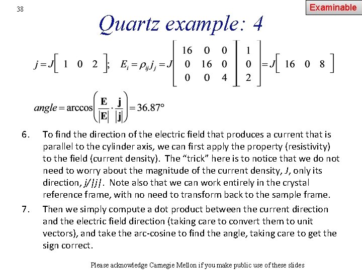
38 6. 7. Quartz example: 4 Examinable To find the direction of the electric field that produces a current that is parallel to the cylinder axis, we can first apply the property (resistivity) to the field (current density). The “trick” here is to notice that we do not need to worry about the magnitude of the current density, J, only its direction, j/|j|. Note also that we can work entirely in the crystal reference frame, with no need to transform back to the sample frame. Then we simply compute a dot product between the current direction and the electric field direction (taking care to convert them to unit vectors), and take the arc-cosine to find the angle, taking care to get the sign correct. Please acknowledge Carnegie Mellon if you make public use of these slides

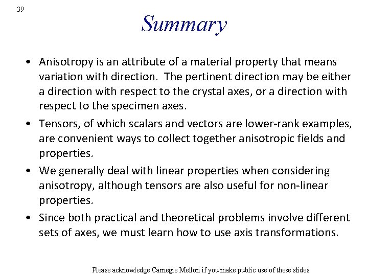
39 Summary • Anisotropy is an attribute of a material property that means variation with direction. The pertinent direction may be either a direction with respect to the crystal axes, or a direction with respect to the specimen axes. • Tensors, of which scalars and vectors are lower-rank examples, are convenient ways to collect together anisotropic fields and properties. • We generally deal with linear properties when considering anisotropy, although tensors are also useful for non-linear properties. • Since both practical and theoretical problems involve different sets of axes, we must learn how to use axis transformations. Please acknowledge Carnegie Mellon if you make public use of these slides

40 Bibliography • R. E. Newnham, Properties of Materials: Anisotropy, Symmetry, Structure, Oxford University Press, 2004, 620. 112 N 55 P. • Nye, J. F. (1957). Physical Properties of Crystals. Oxford, Clarendon Press. • De Graef, M. , lecture notes for 27 -201. • Reid, C. N. (1973). Deformation Geometry for Materials Scientists. Oxford, UK, Pergamon. • Newey, C. and G. Weaver (1991). Materials Principles and Practice. Oxford, England, Butterworth-Heinemann. • Kocks, U. F. , C. Tomé, et al. , Eds. (1998). Texture and Anisotropy, Cambridge University Press, Cambridge, UK. • T. Courtney, Mechanical Behavior of Materials, Mc. Graw-Hill, 0 -07013265 -8, 620. 11292 C 86 M. • Braithwaite, N. and G. Weaver (1991). Electronic Materials. The Open University, England, Butterworth-Heinemann. Please acknowledge Carnegie Mellon if you make public use of these slides

41 Supplemental Slides Please acknowledge Carnegie Mellon if you make public use of these slides

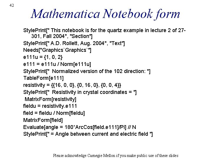
42 Mathematica Notebook form Style. Print[" This notebook is for the quartz example in lecture 2 of 27301, Fall 2004", "Section"] Style. Print[" A. D. Rollett, Aug. 2004", "Text"] Needs["Graphics`"] e 111 u = {1, 0, 2} e 111 = e 111 u / Norm[e 111 u] Style. Print[" Normalized version of the 102 direction: "] Table. Form[e 111] resistivity = {{16, 0, 0}, {0, 16, 0}, {0, 0, 4}} Style. Print[" Resistivity in crystal coordinates = "] Matrix. Form[resistivity] fieldu = resistivity. e 111 field = fieldu / Norm[fieldu] Matrix. Form[field] Evaluate[angle = 180*Arc. Cos[field. e 111]/Pi] // N Style. Print[" = Angle between current and electric field "] Please acknowledge Carnegie Mellon if you make public use of these slides

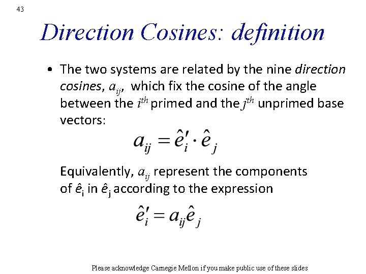
43 Direction Cosines: definition • The two systems are related by the nine direction cosines, aij, which fix the cosine of the angle between the ith primed and the jth unprimed base vectors: Equivalently, aij represent the components of êi in êj according to the expression Please acknowledge Carnegie Mellon if you make public use of these slides

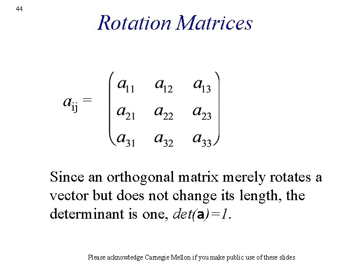
44 Rotation Matrices aij = Since an orthogonal matrix merely rotates a vector but does not change its length, the determinant is one, det(a)=1. Please acknowledge Carnegie Mellon if you make public use of these slides

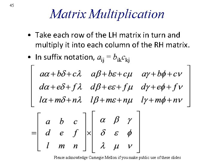
45 Matrix Multiplication • Take each row of the LH matrix in turn and multiply it into each column of the RH matrix. • In suffix notation, aij = bikckj Please acknowledge Carnegie Mellon if you make public use of these slides

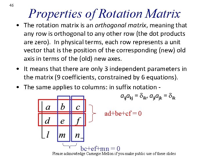
46 Properties of Rotation Matrix • The rotation matrix is an orthogonal matrix, meaning that any row is orthogonal to any other row (the dot products are zero). In physical terms, each row represents a unit vector that is the position of the corresponding (new) old axis in terms of the (old) new axes. • It means that there are only 3 independent parameters in the matrix (9 coefficients, constrained by 6 equations). • The same applies to columns: in suffix notation aijakj = dik, ajiajk = dik ad+be+cf = 0 bc+ef+mn = 0 Please acknowledge Carnegie Mellon if you make public use of these slides

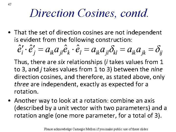
47 Direction Cosines, contd. • That the set of direction cosines are not independent is evident from the following construction: Thus, there are six relationships (i takes values from 1 to 3, and j takes values from 1 to 3) between the nine direction cosines, and therefore, as stated above, only three are independent, exactly as expected for a rotation. • Another way to look at a rotation: combine an axis (described by a unit vector with two parameters) and a rotation angle (one more parameter, for a total of 3). Please acknowledge Carnegie Mellon if you make public use of these slides

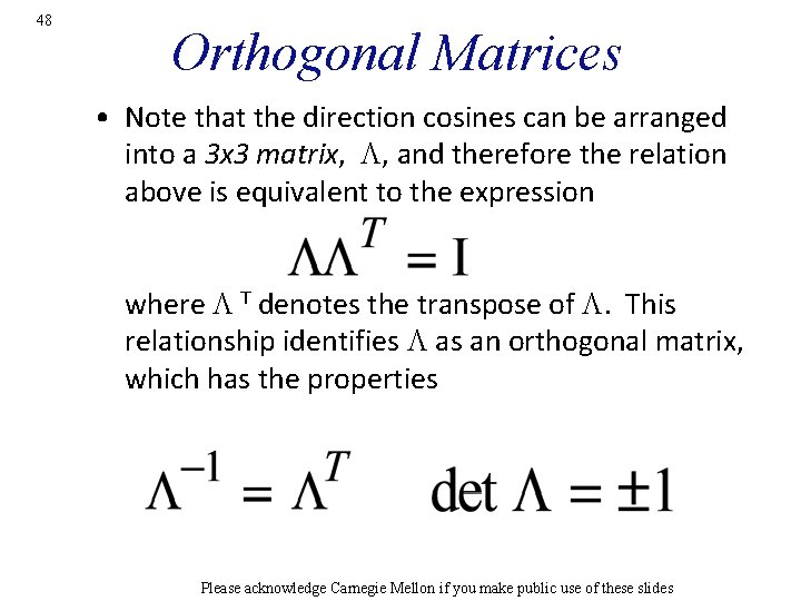
48 Orthogonal Matrices • Note that the direction cosines can be arranged into a 3 x 3 matrix, L, and therefore the relation above is equivalent to the expression where L T denotes the transpose of L. This relationship identifies L as an orthogonal matrix, which has the properties Please acknowledge Carnegie Mellon if you make public use of these slides

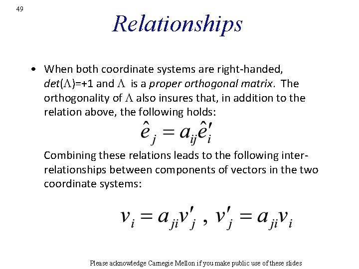
49 Relationships • When both coordinate systems are right-handed, det(L)=+1 and L is a proper orthogonal matrix. The orthogonality of L also insures that, in addition to the relation above, the following holds: Combining these relations leads to the following interrelationships between components of vectors in the two coordinate systems: Please acknowledge Carnegie Mellon if you make public use of these slides

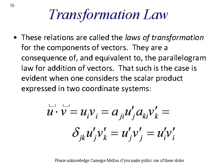
50 Transformation Law • These relations are called the laws of transformation for the components of vectors. They are a consequence of, and equivalent to, the parallelogram law for addition of vectors. That such is the case is evident when one considers the scalar product expressed in two coordinate systems: Please acknowledge Carnegie Mellon if you make public use of these slides

51 Invariants Thus, the transformation law as expressed preserves the lengths and the angles between vectors. Any function of the components of vectors which remains unchanged upon changing the coordinate system is called an invariant of the vectors from which the components are obtained. The derivations illustrate the fact that the scalar product is an invariant of and. Other examples of invariants include the vector product of two vectors and the triple scalar product of three vectors. The reader should note that the transformation law for vectors also applies to the components of points when they are referred to a common origin. Please acknowledge Carnegie Mellon if you make public use of these slides

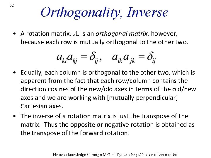
52 Orthogonality, Inverse • A rotation matrix, L, is an orthogonal matrix, however, because each row is mutually orthogonal to the other two. • Equally, each column is orthogonal to the other two, which is apparent from the fact that each row/column contains the direction cosines of the new/old axes in terms of the old/new axes and we are working with [mutually perpendicular] Cartesian axes. • The inverse of a rotation matrix is just the transpose of the matrix. Thus the opposite or negative rotation is obtained as the transpose of the forward rotation. Please acknowledge Carnegie Mellon if you make public use of these slides