Weather Forecasting AK 13 Methods of Forecasting Persistence
 Methods of Forecasting Persistence, Climatology, Trend, Analog, and Numerical Weather")


 • Persistence (What happens today will")


 into the model")


 Nowcast")
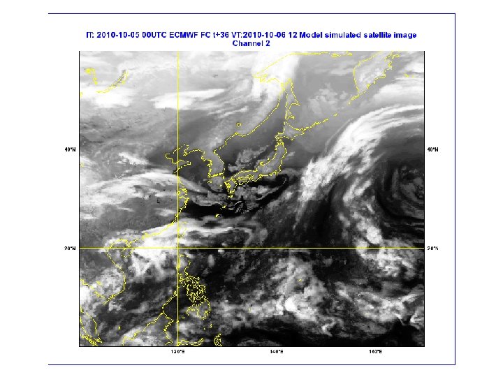
, ECMWF (Europe), GFS (NOAA NCEP), UKMET, Canada and")

 Creates a subgrid scale forecast Captures resolution by doing statistics")
 12 hr")


 • Contains a seamless mosaic of NWS digital forecasts")

- Slides: 60
Weather Forecasting (AK 13) Methods of Forecasting Persistence, Climatology, Trend, Analog, and Numerical Weather Prediction (NWP) NWP Process: -Weather Observations -Data Assimilation -Forecast Model Integration -Interpretation Modern Numerical Weather Prediction Models Short-Range Forecast Models Medium-Range Forecast Models Nowcasting Forecasts of Forecast Accuracy: Ensemble Forecasting
1904 Vilhelm Bjerknes first recognized that numerical weather prediction was possible in principle in 1904. He proposed that weather prediction could be seen as essentially an initial value problem in mathematics, since equations govern how meteorological variables change with time, if we know the initial condition of the atmosphere, we can solve the equations to obtain new values of those variables at a later time (i. e. , make a forecast). Vilhem Frimann Koren Bjerknes (1862 -1951) Vilhelm Bjerknes is considered to be the father of modern meteorology. He led the Bergen School, a talented group of young scientists who made fundamental advances in understanding the weather. From Prof Chuck Wash
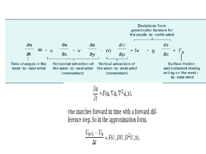
NWP Primitive Equations The primitive equations describe flow on the sphere under the assumptions that vertical motion is much smaller than horizontal motion and that the layer depth is small compared to the radius of the sphere. .
1913 -1916 Lewis Richardson, following Bjerknes’ suggestion, devises numerical methods to solve the system of equations. Lewis Fry Richardson (1881 -1953) Richardson, a brilliant British mathematician, spent almost three years developing the techniques and procedures to solve the equations. It took six weeks to produce a six hour forecast, and the results were very poor. Most of the calculations were performed in a hay loft where Richardson was assigned as an ambulance driver in France during The First World War. A dedicated pacifist, Richardson left meteorology for good when the British government transferred the meteorology office to the War Department shortly after the war. Richardson published a book describing his experiment in 1922. In it, he imagined that, someday, vast numbers of people working on parts of the equations in a huge building could produce weather forecasts in a timely fashion. From Prof Chuck Wash
1947 -1950 1947 -1948 – Jule Charney and Ragnar Fjortoft developed a simplified, filtered system of equations for weather forecasting. 1948 – John Von Neumann developed the first stored program Jule Gregory Charney 1917 -1981 computer (ENIAC). 1950 – Charney, Fjortoft, and von Neumann produce the first successful computer weather forecast. The Birth of computer based Numerical Weather Prediction (NWP) This project was funded by the U. S. Navy through the Office of Naval Research Von Neumann with ENIAC…. which occupied a 30’X 50’ room… but can now be replicated on a single chip… From Prof Chuck Wash “ENIAC-on-a-chip”
LTJG Harry Nicholson 1960 Spanagel Hall room 101 Spanagel Hall Room 101 • Installation of the Navy's First Supercomputer The CDC 1604 pictures show the installation and use of the Navy's first supercomputer, which was installed in 1960 by a team including Seymour Cray himself. "World's first all-solid-state computer -- Model 1, Serial No. 1 of Control Data Corporation's CDC 1604 -- designed, built and personally certified in the lobby of Spanagel Hall (room 101) by the legendary Seymour Cray. "
Methods of Forecasting • Climatology (Long term average) • Persistence (What happens today will happen tomorrow) • Trend (short period NOWCAST) (speed, size, intensity, and direction unchanged) • Analog (Assumes that history repeats itself and weather changes over time) • Conceptual Models (Dynamic description of evolution of weather phenomena) • Numerical Weather Prediction (NWP) Models
Forecast Error The current NWP predictability barrier for the atmosphere is ~14 days. Persistence Climatology Error Forecast Models NWP Ensemble Models 7 days Smart Climo 14 days Human Value added (decreasing) Better Remote sensing data and smarter climo TIME
Factors that determine predictability Model Initial Condition Uncertainty - Lack of full observational coverage at every point in model - Observations are not measured to a infinite degree of precision Model Uncertainty - Model formulation: Uncertainties in parameterizations - Model Processing Resolution precision ≠ accuracy - Equations used do not fully capture processes in atmosphere Nonlinear Dynamics in the atmosphere and oceans - moisture - tropical influences Chaos Theory: small differences in initial state can lead to large differences later. NWP ~ 14 day limit with current methods
Characteristics of a Chaotic System Sensitive to Initial Conditions Aperiodic: Solutions never repeat exactly, but may appear similar Courtesy Maj Eckel
Model Definition: A description of observed behavior, simplified by ignoring certain details, which allows complex systems to be understood and their behavior predicted within the scope of the model. Some Reasons for Model Error 1. Model Resolution is not sufficient to capture all features in the atmosphere. 2. Initial Observations are not available at every point in the atmosphere. 3. The observational data can not be measured to an infinite degree of Precision 4. Equations used by a model do not fully capture processes in the atmosphere.
Old Method of Data Assimilation
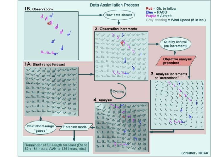
Data Assimilation Bring all the data (spread in time and space) into the model Indirect observations Data void areas use previous forecasts Create the Best Initial Conditions for the Model From Capt. Gunderson
Chaff ?
Data Assimilation Filtering out the Bad data Bad Good 8 hr fcst took 6 weeks to calculate & failed LF Richardson 1922 human computer http: //www. earthsimulator. org. uk/launch. php
1999 French Wind Storm Don’t Filter out the Good Data • Bad Forecast Better Forecast Observations were 'thrown away' as the computer assumed that they were 'wrong' ("quality control")!
Combination of satellite with ground based data is providing global data coverage nearly continuously. Data counts reached are in the tens of millions daily.
Data Assimilation -Quality Control & Weights -Objective analysis vertical and horizontal resolution selected Next Start The Model Initialization of NWP Model Balance, spatial & temporal
Forecast Error The current NWP predictability barrier for the atmosphere is ~14 days. Persistence Climatology Error 7 days Smart Climo Model Initialization Forecast Models NWP Ensemble Models 14 days TIME
Model Topography X X X X Global Model Grid points X X
27 km and 3 km resolution 81 times more grid points 3 km grid
Naturally, one of the limits of models is to properly depict the physical processes that are associated with air flow over or along complex or steep terrain. Here is an comparison of model terrain (colors) with actual terrain.
Improved Marine Forecast of SST with higher res.
Takes at least 5 grid points to define a feature in a grid point model
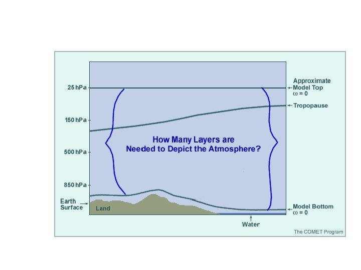
Vertical Levels: -More Near Surface for Moisture & Heat transfer -Less resolution needed ~600 -to ~300 mb -Increases resolution needed near tropopause for Jet stream AFWA MM 5 15 km grid resolution
Sigma Coordinate Pressure ----------Surface Pressure
Model Parameterization When models cannot resolve feature and/or processes that occur within a single grid box they are parameterized. Model the effect of process rather than process itself
40 km
IBM Blue Gene L 2008 Lawrence Livermore Labs 106, 498 nodes NCEP/NOAA 2015 Linux Cluster IBM/CRAY-XC 40
Types of Models • • Global Models Mesoscale-Nested Regional Models Statistical Models (MOS) Nowcast Models Trajectory and Dispersion Models Hysplit Ensemble Models Wave Models Adjoint Models (look back in time)
Meteorological Models Global • NAVGEM (Navy), ECMWF (Europe), GFS (NOAA NCEP), UKMET, Canada and many others • • Resolution ~10 to 100 km 0 to 16 (32) Day Forecast 1 - 6 hour output Interval Run every 6 or 12 hours Regional/Local • COAMPS (Navy), MM 5 (Portable), RUC/RAP (NOAA NCEP) , WRF (NOAA NCEP) • • • Resolution 1 to 30 km 0 to 4 Day Forecast 1 - 3 hour output interval • Run every 1 to 6 hours
Global or Regional Model
Model Output Statistics (MOS) Creates a subgrid scale forecast Captures resolution by doing statistics
Seattle MOS www. meted. ucar. edu Fcsting in the West (B. Colman) 12 hr 30 hr
Cathy Kessinger et al. , NCAR
Hysplit & Cal Puff Trajectory Model and Dispersion Model
John Merrill, University Rhode Is.
Iceland Volcano halts Europe flights 16, 000 Eur flights canceled on Apr 16 th 2010 NASA-Terra 11: 39 z 15 April 2010
Encompassing Forecast Uncertainty An analysis produced to run a model is somewhere in a cloud of likely states. 12 h forecast 12 h verification T T 24 h forecast 48 h forecast 36 h forecast Nonlinearities drive apart the forecast trajectory and true trajectory 24 h (i. e. , Chaos Theory) verification T The true state of the atmosphere exists as a single point that we never know exactly. 36 h verification T 48 h verification T
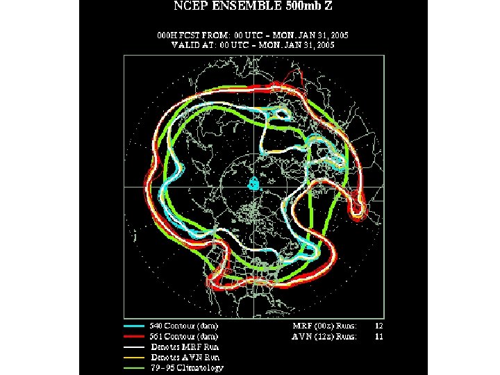
Encompassing Forecast Uncertainty An ensemble of likely analyses leads to an ensemble of likely forecasts T An aly sis R egi on T Ensemble Forecasting: -- Encompasses truth -- Reveals uncertainty -- Yields probabilistic information Courtesy Maj Eckel 48 h forecast Region
Hurricane Frances Ensemble Forecast Problems with tropical influences in mid latitude forecasts and vice versa.
Frances Mean Ensemble and Analysis
An Example of an Ensemble Forecast
NCEP ENSEMBLE FORECAST 6 day Initial Conditions NCEP web training material link Day 15
Wave Forecasts AVN+GDFL Floyd and Gert Sept. 1999
Katrina WW 3 05/08/28/18 z Significant Wave Height = avg height of 1/3 rd largest
Adjoint Models Small inaccuracies in sensitive regions can amplify rapidly 48 Hour Forecast Sensitivity 72 Hour Forecast Sensitivity Adjoint Model: Maps a sensitivity gradient vector from a forecast time, to an earlier time, which can be the initial time of a forecast trajectory. www. nrlmry. navy. mil/projects/adap. html www. nrlmry. navy. mil/~langland/adap_about. html
Checking the models
Model Verification UW Model 1 Model 3 Model 2 Analysis
NWS Traditional Forecasting Process – Schedule Driven – Product Oriented – Labor Intensive National Centers Model Guidance Field Offices National Centers Type Text Products Generate Graphical Products TODAY. . . RAIN LIKELY. SNOW LIKELY ABOVE 2500 FEET. SNOW ACCUMULATION BY LATE AFTERNOON 1 TO 2 INCHES ABOVE 2500 FEET. COLDER WITH HIGHS 35 TO 40. SOUTHEAST WIND 5 TO 10 MPH SHIFTING TO THE SOUTHWESTEARLY THIS AFTERNOON. MARYLAND EASTERN SHORE CHANCE OF PRECIPITATION 70%. EASTON PTCLDY CLOUDY PTCLDY SUNNY PTCLDY 60/52 63/54 65/47 55/40 55/37 50/33 POP 20 POP 10 » » » » » » » » » » » » » » » » » » » » » U. S. Drought Monitor Threats Assessments Excessive Heat Products
New Forecasting Process National Centers Model Guidance – Interactive – Collaborative – Information Oriented Grids Field Offices Local Digital Forecast Database Collaborate National Centers Data and Science Focus NWS Automated Products LY. LIKEOVE B. RAIN LY A AY. . TODOW LIKE. SNOWBY SN 0 FEET ATION N 1 250 CUMULERNOOOVE AC E AFT ES AB DER LAT 2 INCH. COL TO 40. TO 0 FEETHS 35 D 5 250 H HIG ST WINTING WITUTHEAH SHIF SO 10 MP Y ARL TO THE STE N. TO UTHWE RNOO SO IS AFTEOF 0%. 7 N H E T ANC ATIO CH ECIPIT PR Digital Text Graphic Voice User-Generated Products National Digital Forecast Database
Editing: manually The pencil tool allows for quick “stretching” of values. The GFE then recalculates the grid.
National Digital Forecast Database (NDFD) • Contains a seamless mosaic of NWS digital forecasts • Is available to all users and partners – public and private • Allows users and partners to create a wide range of text, graphic, and image products