Forecasting OBJECTIVES Demand Management Qualitative Forecasting Methods Simple

Forecasting

• • • OBJECTIVES Demand Management Qualitative Forecasting Methods Simple & Weighted Moving Average Forecasts Basic Exponential Smoothing with trend Web-Based Forecasting

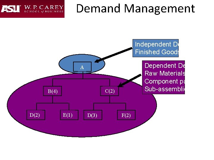
Demand Management Independent Demand: Finished Goods Dependent Demand: Raw Materials, Component parts, Sub-assemblies, etc. A C(2) B(4) D(2) E(1) D(3) F(2)

Independent Demand: What a firm can do to manage it? • Can take an active role to influence demand • Can take a passive role and simply respond to demand

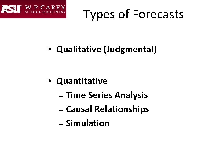
Types of Forecasts • Qualitative (Judgmental) • Quantitative – Time Series Analysis – Causal Relationships – Simulation

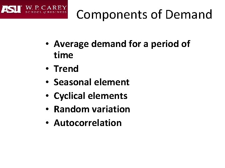
Components of Demand • Average demand for a period of time • Trend • Seasonal element • Cyclical elements • Random variation • Autocorrelation

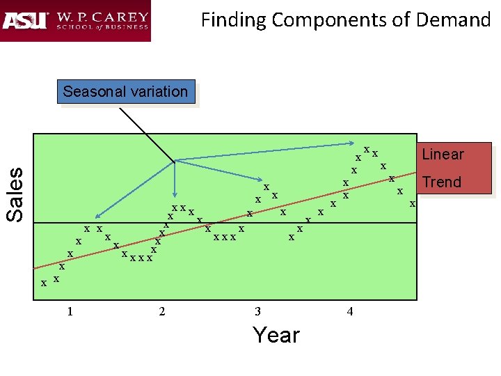
Finding Components of Demand Sales Seasonal variation x x xx x x x xxxx 1 2 x x x 3 Year x x x x x 4 Linear x x Trend x

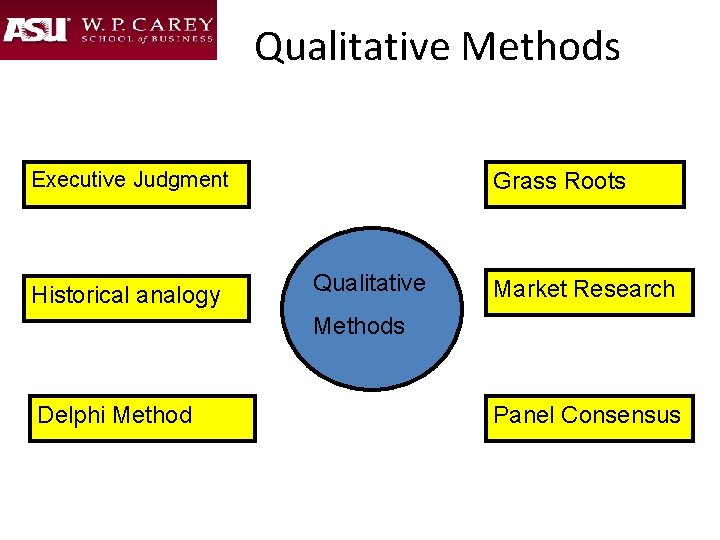
Qualitative Methods Executive Judgment Historical analogy Grass Roots Qualitative Market Research Methods Delphi Method Panel Consensus

Delphi Method l. Choose the experts to participate representing a variety of knowledgeable people in different areas 2. Through a questionnaire (or E-mail), obtain forecasts (and any premises or qualifications for the forecasts) from all participants 3. Summarize the results and redistribute them to the participants along with appropriate new questions 4. Summarize again, refining forecasts and conditions, and again develop new questions 5. Repeat Step 4 as necessary and distribute the final results to all participants

Time Series Analysis • Time series forecasting models try to predict the future based on past data • You can pick models based on: 1. Time horizon to forecast 2. Data availability 3. Accuracy required 4. Size of forecasting budget 5. Availability of qualified personnel

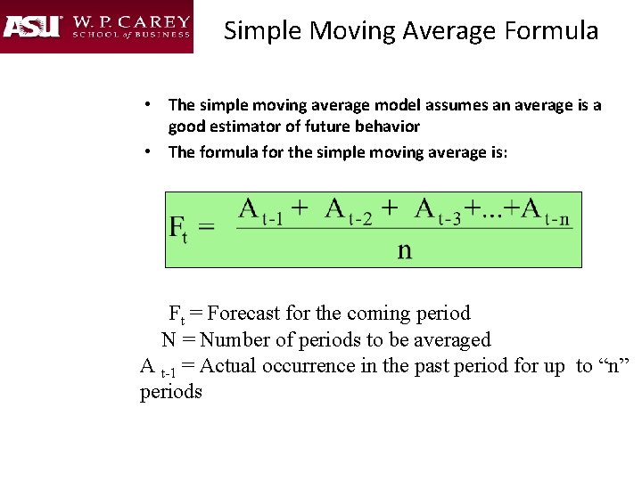
Simple Moving Average Formula • The simple moving average model assumes an average is a good estimator of future behavior • The formula for the simple moving average is: Ft = Forecast for the coming period N = Number of periods to be averaged A t-1 = Actual occurrence in the past period for up to “n” periods

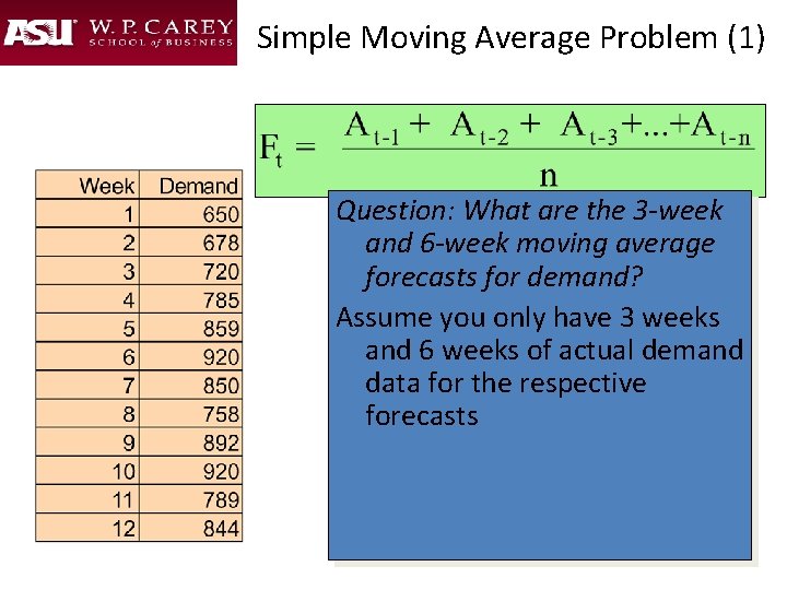
Simple Moving Average Problem (1) Question: What are the 3 -week and 6 -week moving average forecasts for demand? Assume you only have 3 weeks and 6 weeks of actual demand data for the respective forecasts

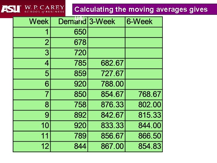
Calculating the moving averages gives us:

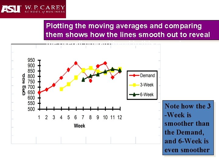
Plotting the moving averages and comparing them shows how the lines smooth out to reveal the overall upward trend in this example Note how the 3 -Week is smoother than the Demand, and 6 -Week is even smoother

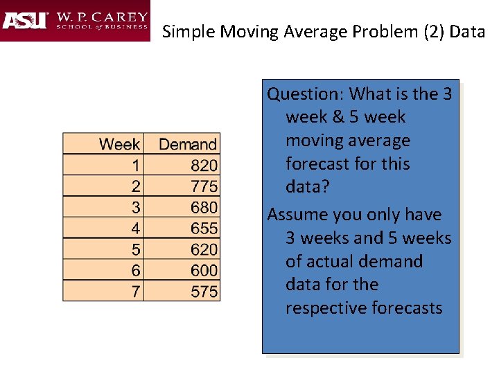
Simple Moving Average Problem (2) Data Question: What is the 3 week & 5 week moving average forecast for this data? Assume you only have 3 weeks and 5 weeks of actual demand data for the respective forecasts

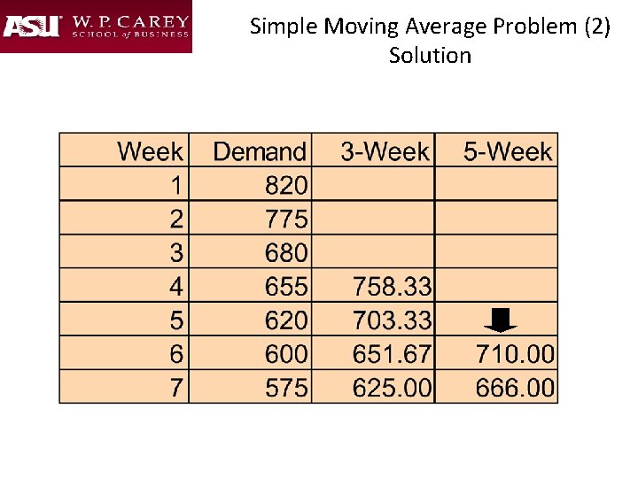
Simple Moving Average Problem (2) Solution

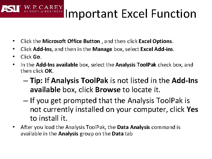
Important Excel Function • • Click the Microsoft Office Button , and then click Excel Options. Click Add-Ins, and then in the Manage box, select Excel Add-ins. Click Go. In the Add-Ins available box, select the Analysis Tool. Pak check box, and then click OK. – Tip: If Analysis Tool. Pak is not listed in the Add-Ins available box, click Browse to locate it. – If you get prompted that the Analysis Tool. Pak is not currently installed on your computer, click Yes to install it. • After you load the Analysis Tool. Pak, the Data Analysis command is available in the Analysis group on the Data tab

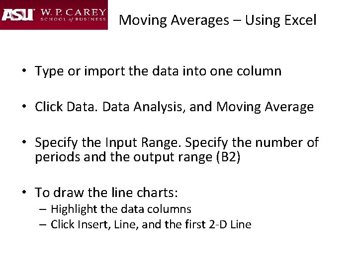
Moving Averages – Using Excel • Type or import the data into one column • Click Data Analysis, and Moving Average • Specify the Input Range. Specify the number of periods and the output range (B 2) • To draw the line charts: – Highlight the data columns – Click Insert, Line, and the first 2 -D Line

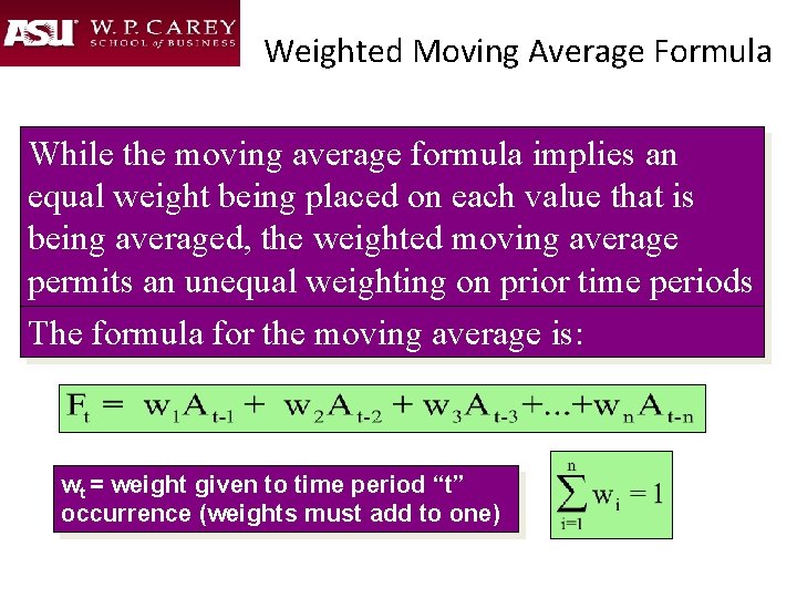
Weighted Moving Average Formula While the moving average formula implies an equal weight being placed on each value that is being averaged, the weighted moving average permits an unequal weighting on prior time periods The formula for the moving average is: wt = weight given to time period “t” occurrence (weights must add to one)

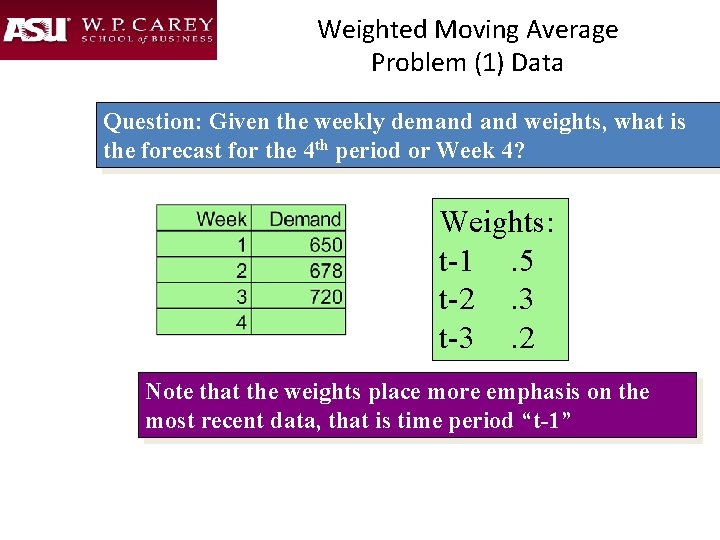
Weighted Moving Average Problem (1) Data Question: Given the weekly demand weights, what is the forecast for the 4 th period or Week 4? Weights: t-1. 5 t-2. 3 t-3. 2 Note that the weights place more emphasis on the most recent data, that is time period “t-1”

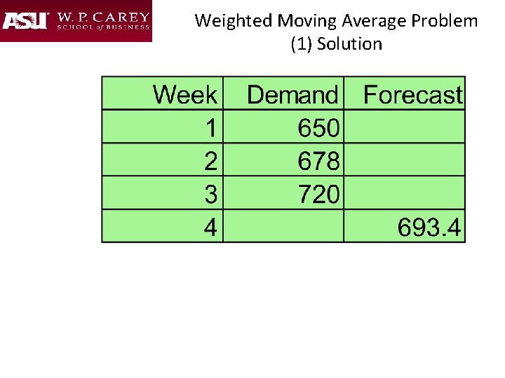
Weighted Moving Average Problem (1) Solution

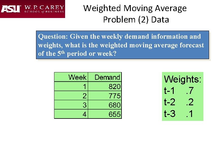
Weighted Moving Average Problem (2) Data Question: Given the weekly demand information and weights, what is the weighted moving average forecast of the 5 th period or week? Weights: t-1. 7 t-2. 2 t-3. 1

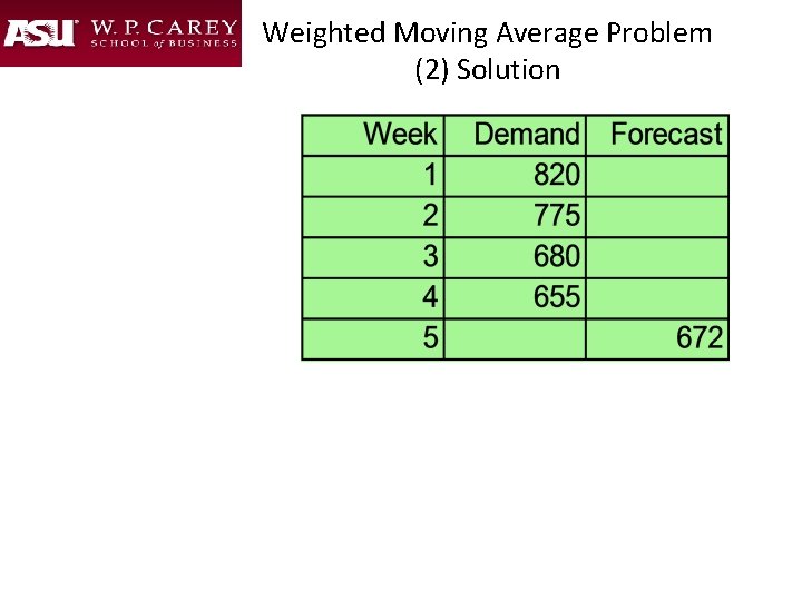
Weighted Moving Average Problem (2) Solution

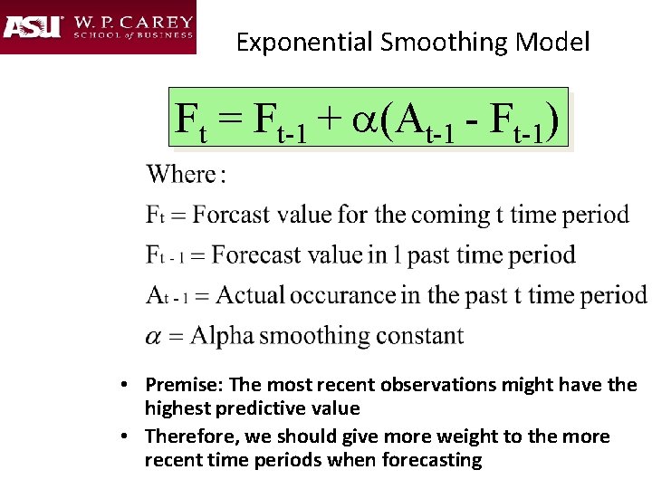
Exponential Smoothing Model Ft = Ft-1 + a(At-1 - Ft-1) • Premise: The most recent observations might have the highest predictive value • Therefore, we should give more weight to the more recent time periods when forecasting

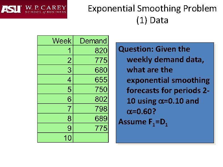
Exponential Smoothing Problem (1) Data Question: Given the weekly demand data, what are the exponential smoothing forecasts for periods 210 using a=0. 10 and a=0. 60? Assume F 1=D 1

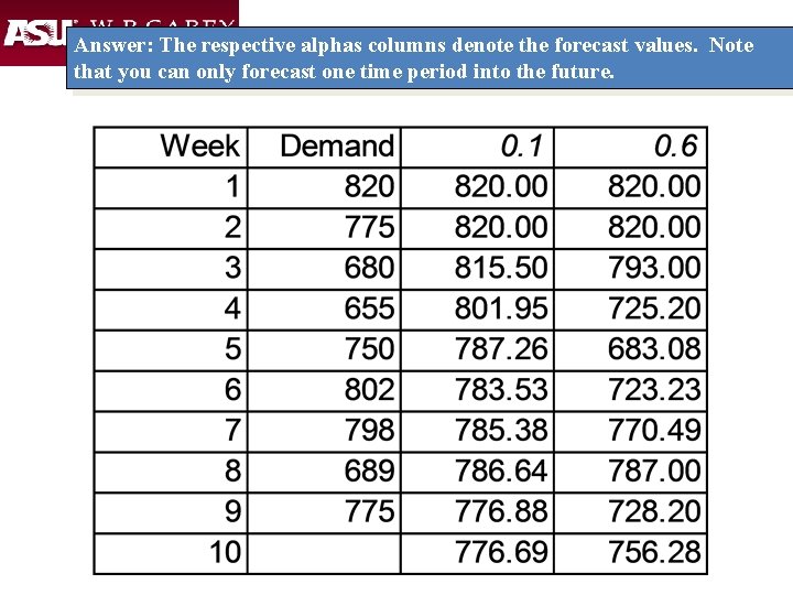
Answer: The respective alphas columns denote the forecast values. Note that you can only forecast one time period into the future.

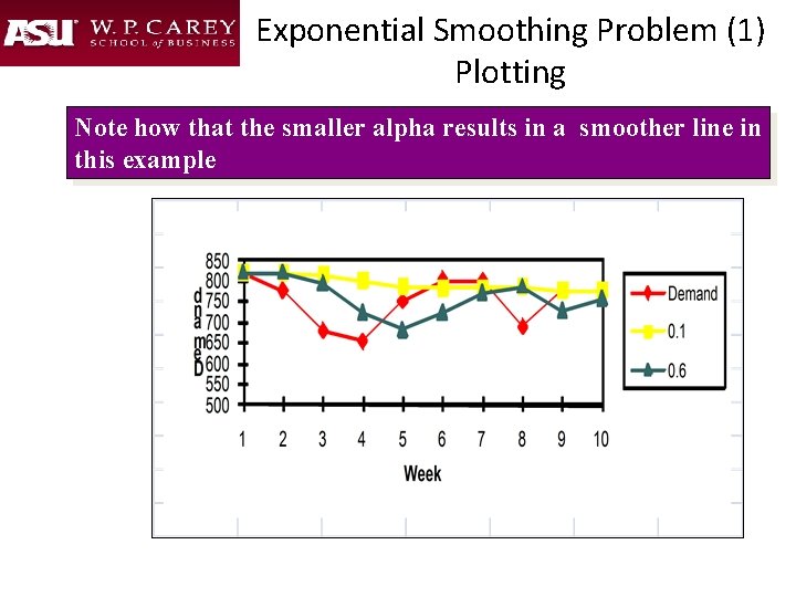
Exponential Smoothing Problem (1) Plotting Note how that the smaller alpha results in a smoother line in this example

Exponential Smoothing – Using Excel • Type or import the data into one column • Click Data, Data Analysis, and Exponential Smoothing • Specify the Input Range (extend to include all periods to be forecasted). Type the Smoothing or Damping factor. Specify the output range e. g. (B 1) • To calculate the second exponentially smoothed time series, specify the new smoothing factor, and output range e. g. (C 1)

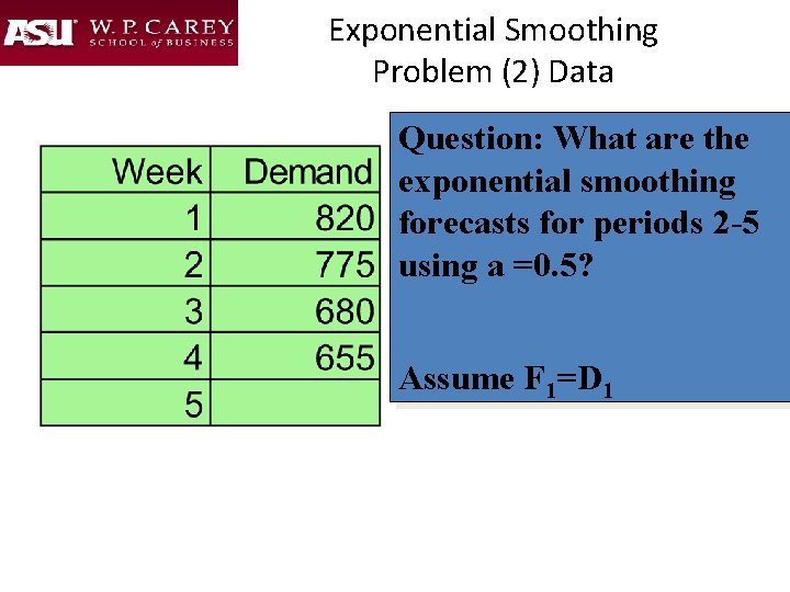
Exponential Smoothing Problem (2) Data Question: What are the exponential smoothing forecasts for periods 2 -5 using a =0. 5? Assume F 1=D 1

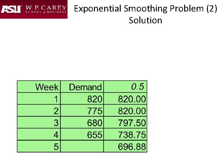
Exponential Smoothing Problem (2) Solution

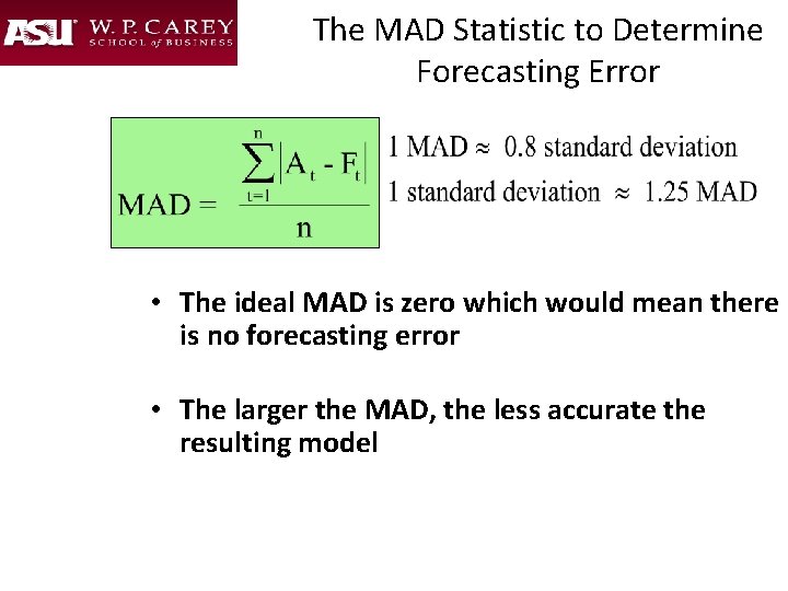
The MAD Statistic to Determine Forecasting Error • The ideal MAD is zero which would mean there is no forecasting error • The larger the MAD, the less accurate the resulting model

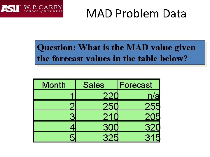
MAD Problem Data Question: What is the MAD value given the forecast values in the table below? Month Sales 1 2 3 4 5 220 250 210 300 325 Forecast n/a 255 205 320 315

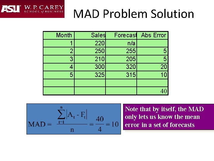
MAD Problem Solution Month 1 2 3 4 5 Sales 220 250 210 300 325 Forecast Abs Error n/a 255 5 205 5 320 20 315 10 40 Note that by itself, the MAD only lets us know the mean error in a set of forecasts

Exponential Smoothing with Trend • Adds a trend adjustment to make the forecast a little more precise • Uses a trend smoothing constant delta (d) • Idea of double smoothing

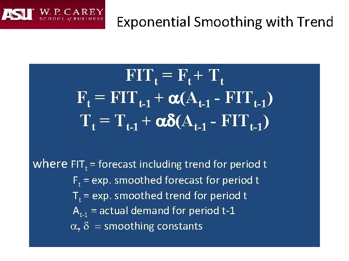
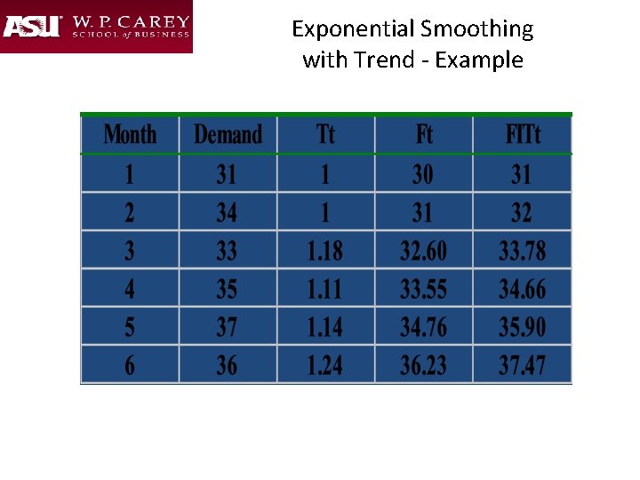
Exponential Smoothing with Trend FITt = Ft + Tt Ft = FITt-1 + a(At-1 - FITt-1) Tt = Tt-1 + ad(At-1 - FITt-1) where FITt = forecast including trend for period t Ft = exp. smoothed forecast for period t Tt = exp. smoothed trend for period t At-1 = actual demand for period t-1 a, d = smoothing constants

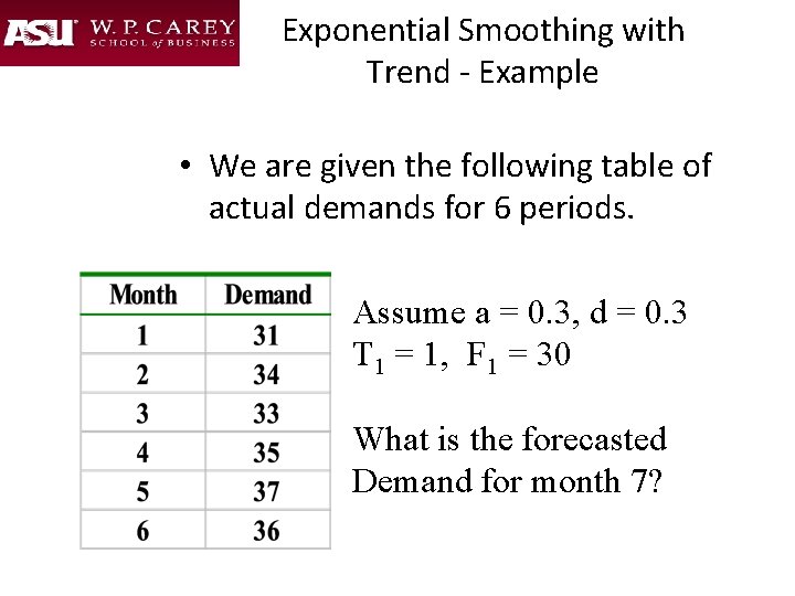
Exponential Smoothing with Trend - Example • We are given the following table of actual demands for 6 periods. Assume a = 0. 3, d = 0. 3 T 1 = 1, F 1 = 30 What is the forecasted Demand for month 7?

Exponential Smoothing with Trend - Example

Exponential Smoothing with Trend - Example

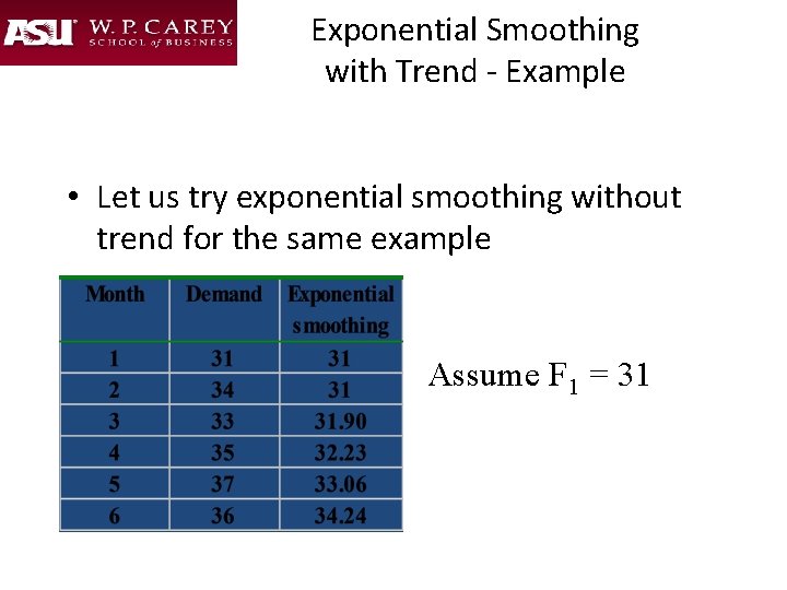
Exponential Smoothing with Trend - Example • Let us try exponential smoothing without trend for the same example Assume F 1 = 31

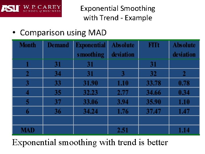
Exponential Smoothing with Trend - Example • Comparison using MAD Exponential smoothing with trend is better

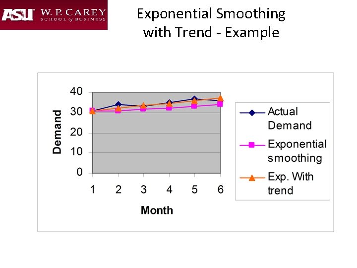
Exponential Smoothing with Trend - Example

Web-Based Forecasting: CPFR • Collaborative Planning, Forecasting, and Replenishment (CPFR) a Web-based tool used to coordinate demand forecasting, production and purchase planning, and inventory replenishment between supply chain trading partners. • Used to integrate the multi-tier or n-Tier supply chain, including manufacturers, distributors and retailers. • CPFR’s objective is to exchange selected internal information to provide for a reliable, longer term future views of demand in the supply chain. • CPFR uses a cyclic and iterative approach to derive consensus forecasts.

Web-Based Forecasting: Steps in CPFR • 1. Creation of a front-end partnership agreement • 2. Joint business planning • 3. Development of demand forecasts • 4. Sharing forecasts • 5. Inventory replenishment

Question Bowl Which of the following is a classification of a basic type of forecasting? a. b. c. d. e. Transportation method Simulation Linear programming All of the above None of the above

Question Bowl Which of the following is an example of a “Qualitative” type of forecasting technique or model? a. Grass roots b. Market research c. Panel consensus d. All of the above e. None of the above

Question Bowl Which of the following is an example of a “Time Series Analysis” type of forecasting technique or model? a. Simulation b. Exponential smoothing c. Panel consensus d. All of the above e. None of the above

Question Bowl Which of the following is a reason why a firm should choose a particular forecasting model? a. Time horizon to forecast b. Data availability c. Accuracy required d. Size of forecasting budget e. All of the above

Question Bowl Which of the following are ways to choose weights in a Weighted Moving Average forecasting model? a. Cost b. Experience c. Trial and error d. Only b and c above e. None of the above

Question Bowl Which of the following are reasons why the Exponential Smoothing model has been a well accepted forecasting methodology? a. It is accurate b. It is easy to use c. Computer storage requirements are small d. All of the above e. None of the above

Question Bowl The value for alpha or α must be between which of the following when used in an Exponential Smoothing model? a. 1 to 10 b. 1 to 2 c. 0 to 1 d. -1 to 1 e. Any number at all

Question Bowl Which of the following are sources of error in forecasts? a. Bias b. Random c. Employing the wrong trend line d. All of the above e. None of the above

Question Bowl Which of the following would be the “best” MAD values in an analysis of the accuracy of a forecasting model? a. 1000 b. 100 c. 10 d. 1 e. 0