Todays topics Impaired wandering Instant Insanity 1950 s

Today’s topics • • Impaired wandering Instant Insanity 1950 s TV Dating Final Exam review Comp. Sci 102 18. 1

Getting back home - Lost in a city, you want to get back to your hotel. How should you do this? Depth First Search: requires a good memory and a piece of chalk

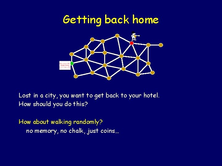
Getting back home - Lost in a city, you want to get back to your hotel. How should you do this? How about walking randomly? no memory, no chalk, just coins…

Will this work? When will I get home? I have a curfew of 10 PM!

Will this work? Is Pr[ reach home ] = 1? When will I get home? What is E[ time to reach home ]? I have a curfew of 10 PM!

Relax, Bonzo! Yes, Pr[ will reach home ] = 1

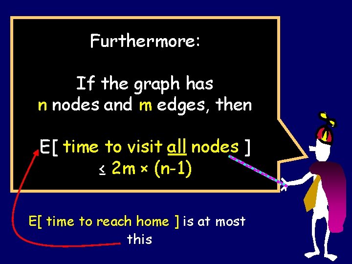
Furthermore: If the graph has n nodes and m edges, then E[ time to visit all nodes ] ≤ 2 m × (n-1) E[ time to reach home ] is at most this

Cover times Let us define a couple of useful things: Cover time (from u) Cu = E [ time to visit all vertices | start at u ] Cover time of the graph: C(G) = maxu { Cu }

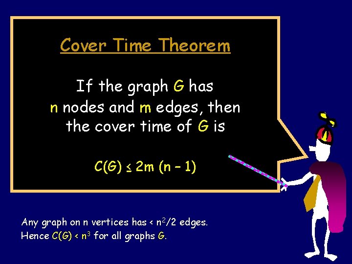
Cover Time Theorem If the graph G has n nodes and m edges, then the cover time of G is C(G) ≤ 2 m (n – 1) Any graph on n vertices has < n 2/2 edges. Hence C(G) < n 3 for all graphs G.

First, let’s prove that Pr[ eventually get home ] = 1

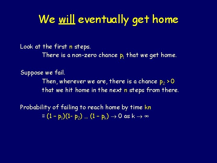
We will eventually get home Look at the first n steps. There is a non-zero chance p 1 that we get home. Suppose we fail. Then, wherever we are, there is a chance p 2 > 0 that we hit home in the next n steps from there. Probability of failing to reach home by time kn = (1 – p 1)(1 - p 2) … (1 – pk) 0 as k ∞

In fact Pr[ we don’t get home by 2 k C(G) steps ] ≤ (½)k Recall: C(G) = cover time of G ≤ 2 m(n-1)

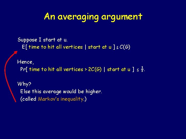
An averaging argument Suppose I start at u. E[ time to hit all vertices | start at u ] ≤ C(G) Hence, Pr[ time to hit all vertices > 2 C(G) | start at u ] ≤ ½. Why? Else this average would be higher. (called Markov’s inequality. )

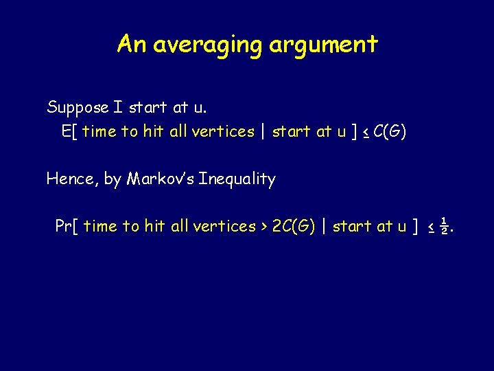
An averaging argument Suppose I start at u. E[ time to hit all vertices | start at u ] ≤ C(G) Hence, by Markov’s Inequality Pr[ time to hit all vertices > 2 C(G) | start at u ] ≤ ½.

so let’s walk some more! Pr [ time to hit all vertices > 2 C(G) | start at u ] ≤ ½. Suppose at time 2 C(G), am at some node v, with more nodes still to visit. Pr [ haven’t hit all vertices in 2 C(G) more time ½. Chance that you failed both times ≤ ¼ ! | start at v ] ≤

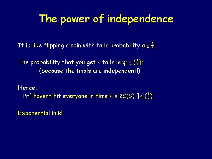
The power of independence It is like flipping a coin with tails probability q ≤ ½. The probability that you get k tails is qk ≤ (½)k. (because the trials are independent!) Hence, Pr[ havent hit everyone in time k × 2 C(G) ] ≤ (½)k Exponential in k!

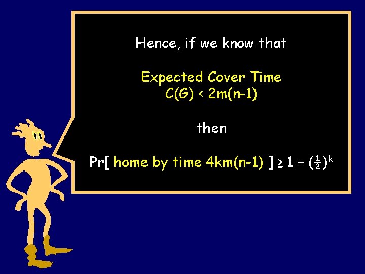
Hence, if we know that Expected Cover Time C(G) < 2 m(n-1) then Pr[ home by time 4 km(n-1) ] ≥ 1 – (½)k

Random walks on infinite graphs

A drunk man will find his way home, but a drunk bird may get lost forever - Shizuo Kakutani

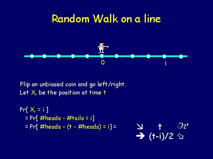
Random Walk on a line 0 i Flip an unbiased coin and go left/right. Let Xt be the position at time t Pr[ Xt = i ] = Pr[ #heads - #tails = i] = Pr[ #heads – (t - #heads) = i] = t /2 t (t-i)/2

Unbiased Random Walk 0 Pr[ X 2 t = 0 ] = 2 t 2 t /2 t Stirling’s approximation: n! = Θ((n/e)n × √n) Hence: (2 n)!/(n!)2 = p £ ( ( 2 en ) 2 n ) p n n £ n) ( ( ) ½ e = Θ(22 n/n ) 2 n

Unbiased Random Walk 0 Pr[ X 2 t = 0 ] = Sterling’s approx. 2 t 2 t ≤ Θ(1/√t) /2 t Y 2 t = indicator for (X 2 t = 0) E[ Y 2 t ] = Θ(1/√t) Z 2 n = number of visits to origin in 2 n steps. E[ Z 2 n ] = E[ t = 1…n Y 2 t ] = Θ(1/√ 1 + 1/√ 2 +…+ 1/√n) = Θ(√n)

In n steps, you expect to return to the origin Θ(√n) times!

Simple Claim Recall: if we repeatedly flip coin with bias p E[ # of flips till heads ] = 1/p. Claim: If Pr[ not return to origin ] = p, then E[ number of times at origin ] = 1/p. Proof: H = never return to origin. T = we do. Hence returning to origin is like getting a tails. E[ # of returns ] = E[ # tails before a head] = 1/p – 1. (But we started at the origin too!)

We will return… Claim: If Pr[ not return to origin ] = p, then E[ number of times at origin ] = 1/p. Theorem: Pr[ we return to origin ] = 1. Proof: Suppose not. Hence p = Pr[ never return ] > 0. E [ #times at origin ] = 1/p = constant. But we showed that E[ Zn ] = Θ(√n) ∞

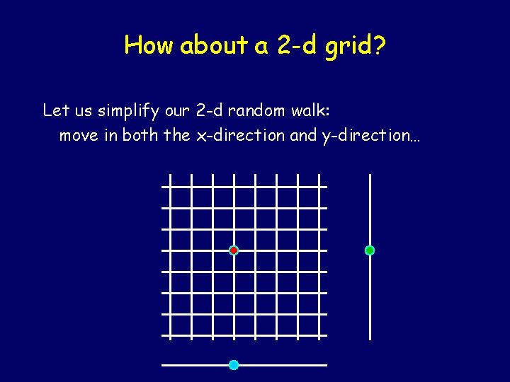
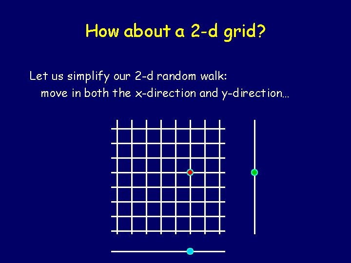
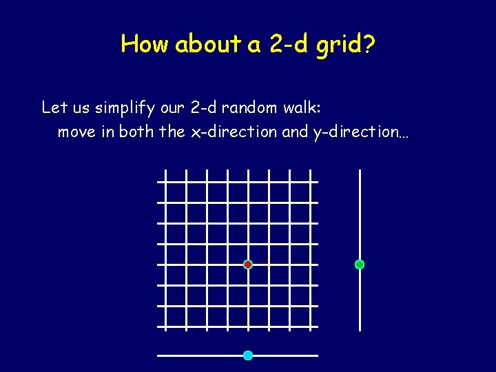
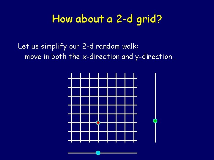
How about a 2 -d grid? Let us simplify our 2 -d random walk: move in both the x-direction and y-direction…

How about a 2 -d grid? Let us simplify our 2 -d random walk: move in both the x-direction and y-direction…

How about a 2 -d grid? Let us simplify our 2 -d random walk: move in both the x-direction and y-direction…

How about a 2 -d grid? Let us simplify our 2 -d random walk: move in both the x-direction and y-direction…

How about a 2 -d grid? Let us simplify our 2 -d random walk: move in both the x-direction and y-direction…

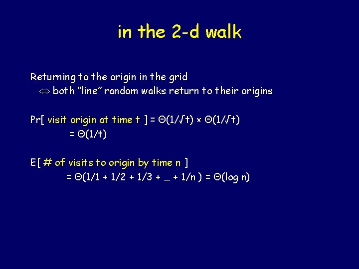
in the 2 -d walk Returning to the origin in the grid both “line” random walks return to their origins Pr[ visit origin at time t ] = Θ(1/√t) × Θ(1/√t) = Θ(1/t) E[ # of visits to origin by time n ] = Θ(1/1 + 1/2 + 1/3 + … + 1/n ) = Θ(log n)

We will return (again!)… Claim: If Pr[ not return to origin ] = p, then E[ number of times at origin ] = 1/p. Theorem: Pr[ we return to origin ] = 1. Proof: Suppose not. Hence p = Pr[ never return ] > 0. E [ #times at origin ] = 1/p = constant. But we showed that E[ Zn ] = Θ(log n) ∞

But in 3 -d Pr[ visit origin at time t ] = Θ(1/√t)3 = Θ(1/t 3/2) limn ∞ E[ # of visits by time n ] < K (constant) Hence Pr[ never return to origin ] > 1/K.

Great Theoretical Ideas In Computer Science Steven Rudich Lecture 11 CS 15 -251 Feb 15, 2005 Spring 2005 Carnegie Mellon University The Mathematics Of 1950’s TV-style Dating: Who wins the battle of the sexes?

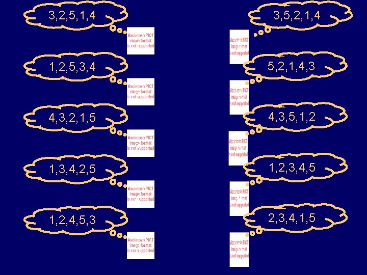
3, 2, 5, 1, 4 3, 5, 2, 1, 4 1 1 5, 2, 1, 4, 3 1, 2, 5, 3, 4 2 2 4, 3, 5, 1, 2 4, 3, 2, 1, 5 3 3 1, 2, 3, 4, 5 1, 3, 4, 2, 5 4 4 2, 3, 4, 1, 5 1, 2, 4, 5, 3 5 5

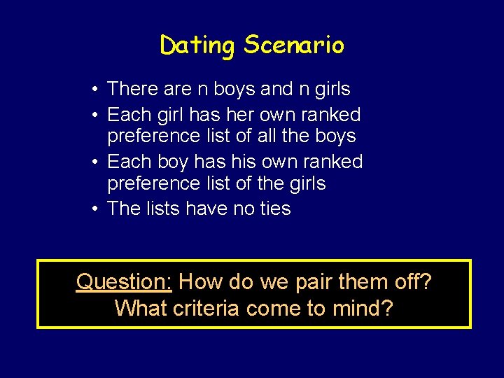
Dating Scenario • There are n boys and n girls • Each girl has her own ranked preference list of all the boys • Each boy has his own ranked preference list of the girls • The lists have no ties Question: How do we pair them off? What criteria come to mind?

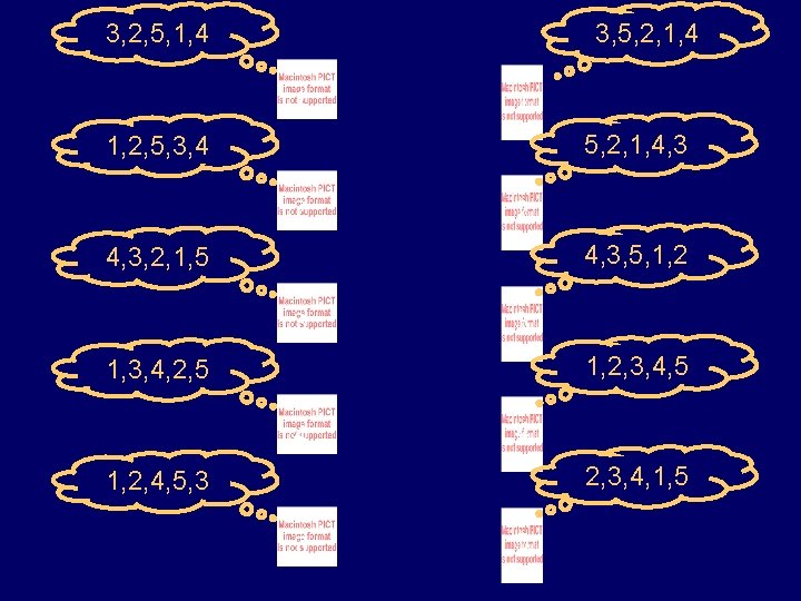
3, 2, 5, 1, 4 3, 5, 2, 1, 4 1 1 5, 2, 1, 4, 3 1, 2, 5, 3, 4 2 2 4, 3, 5, 1, 2 4, 3, 2, 1, 5 3 3 1, 2, 3, 4, 5 1, 3, 4, 2, 5 4 4 2, 3, 4, 1, 5 1, 2, 4, 5, 3 5 5

We will ignore the issue of what is “equitable”!

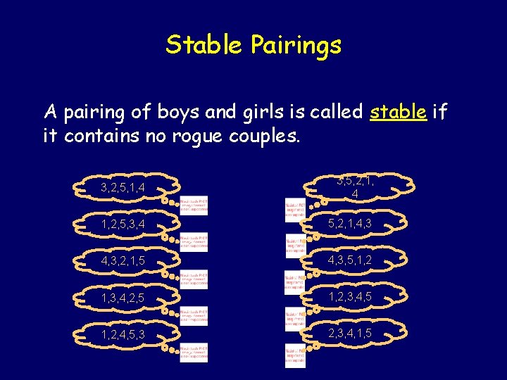
Rogue Couples Suppose we pair off all the boys and girls. Now suppose that some boy and some girl prefer each other to the people to whom they are paired. They will be called a rogue couple.

Why be with them when we can be with each other?

Stable Pairings A pairing of boys and girls is called stable if it contains no rogue couples. 3, 5, 2, 1, 4 3, 2, 5, 1, 4 1 1 5, 2, 1, 4, 3 1, 2, 5, 3, 4 2 2 4, 3, 5, 1, 2 4, 3, 2, 1, 5 3 3 1, 2, 3, 4, 5 1, 3, 4, 2, 5 4 4 2, 3, 4, 1, 5 1, 2, 4, 5, 3 5 5

What use is fairness, if it is not stable? Any list of criteria for a good pairing must include stability. (A pairing is doomed if it contains a rogue couple. ) Any reasonable list of criteria must contain the stability criterion.

The study of stability will be the subject of the entire lecture. We will: • Analyze various mathematical properties of an algorithm that looks a lot like 1950’s dating • Discover the naked mathematical truth about which sex has the romantic edge • Learn how the world’s largest, most successful dating service operates

The Traditional Marriage Algorithm

The Traditional Marriage Algorithm Female Worshipping males String

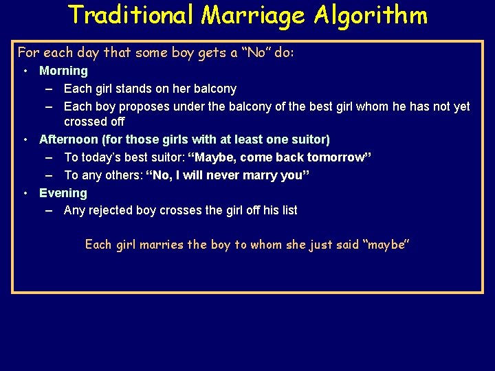
Traditional Marriage Algorithm For each day that some boy gets a “No” do: • Morning – Each girl stands on her balcony – Each boy proposes under the balcony of the best girl whom he has not yet crossed off • Afternoon (for those girls with at least one suitor) – To today’s best suitor: “Maybe, come back tomorrow” – To any others: “No, I will never marry you” • Evening – Any rejected boy crosses the girl off his list Each girl marries the boy to whom she just said “maybe”

Does the Traditional Marriage Algorithm always produce a stable pairing?

Does the Traditional Marriage Algorithm always produce a stable pairing? Wait! There is a more primary question!

Does TMA always terminate? • It might encounter a situation where algorithm does not specify what to do next (core dump error) • It might keep on going for an infinite number of days

Traditional Marriage Algorithm For each day that some boy gets a “No” do: • Morning – Each girl stands on her balcony – Each boy proposes under the balcony of the best girl whom he has not yet crossed off • Afternoon (for those girls with at least one suitor) – To today’s best suitor: “Maybe, come back tomorrow” – To any others: “No, I will never marry you” • Evening – Any rejected boy crosses the girl off his list Each girl marries the boy to whom she just said “maybe”

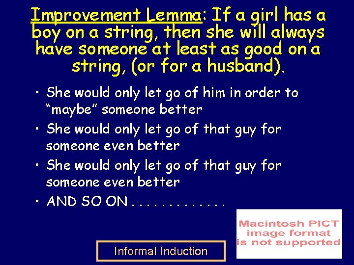
Improvement Lemma: If a girl has a boy on a string, then she will always have someone at least as good on a string, (or for a husband). • She would only let go of him in order to “maybe” someone better • She would only let go of that guy for someone even better • AND SO ON. . . Informal Induction

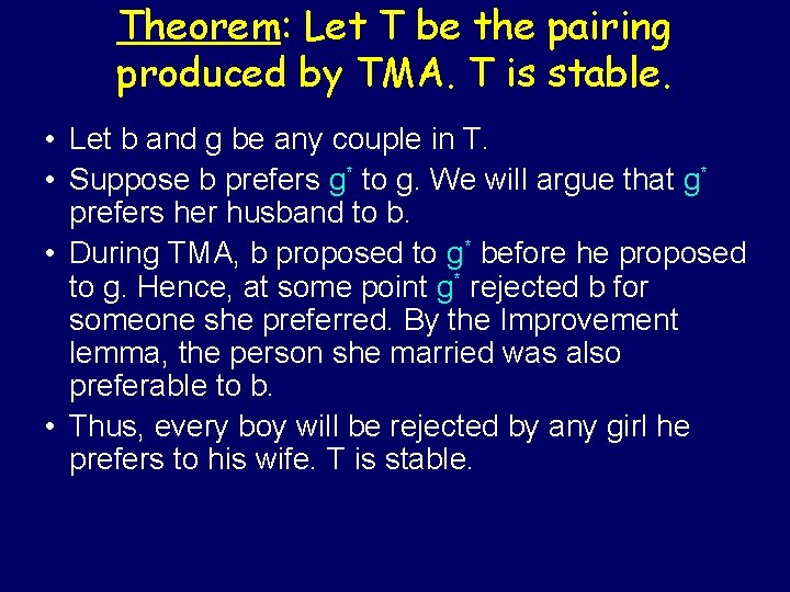
Theorem: Let T be the pairing produced by TMA. T is stable. • Let b and g be any couple in T. • Suppose b prefers g* to g. We will argue that g* prefers her husband to b. • During TMA, b proposed to g* before he proposed to g. Hence, at some point g* rejected b for someone she preferred. By the Improvement lemma, the person she married was also preferable to b. • Thus, every boy will be rejected by any girl he prefers to his wife. T is stable.

Opinion Poll n i f f o r , e t t g e atin b s i d l e o a h h t n r W ditio o tra boys ? the girls

Forget TMA for a moment How should we define what we mean when we say “the optimal girl for boy b”? Flawed Attempt: “The girl at the top of b’s list”

The Optimal Girl A boy’s optimal girl is the highest ranked girl for whom there is some stable pairing in which the boy gets her. She is the best girl he can conceivably get in a stable world. Presumably, she might be better than the girl he gets in the stable pairing output by TMA.

The Pessimal Girl A boy’s pessimal girl is the lowest ranked girl for whom there is some stable pairing in which the boy gets her. She is the worst girl he can conceivably get in a stable world.

Dating Heaven and Hell A pairing is male-optimal if every boy gets his optimal mate. This is the best of all possible stable worlds for every boy simultaneously. A pairing is male-pessimal if every boy gets his pessimal mate. This is the worst of all possible stable worlds for every boy simultaneously.

Dating Heaven and Hell A pairing is male-optimal if every boy gets his optimal mate. Thus, the pairing is simultaneously giving each boy his optimal. Is a male-optimal pairing always stable?

Dating Heaven and Hell A pairing is female-optimal if every girl gets her optimal mate. This is the best of all possible stable worlds for every girl simultaneously. A pairing is female-pessimal if every girl gets her pessimal mate. This is the worst of all possible stable worlds for every girl simultaneously.

The Naked Mathematical Truth! The Traditional Marriage Algorithm always produces a male-optimal, femalepessimal pairing.

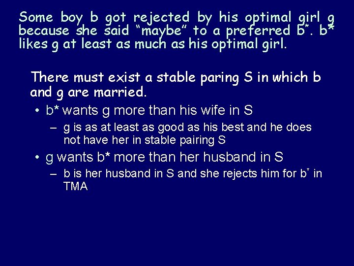
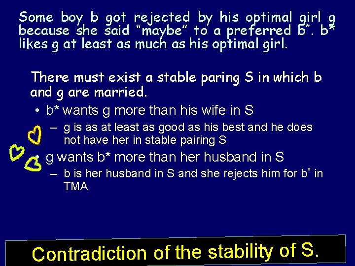
Theorem: TMA produces a male-optimal pairing • Suppose, for a contradiction, that some boy gets rejected by his optimal girl during TMA. Let t be the earliest time at which this happened. • In particular, at time t, some boy b got rejected by his optimal girl g because she said “maybe” to a preferred b*. By the definition of t, b* had not yet been rejected by his optimal girl. • Therefore, b* likes g at least as much as his optimal.

Some boy b got rejected by his optimal girl g because she said “maybe” to a preferred b*. b* likes g at least as much as his optimal girl. There must exist a stable paring S in which b and g are married. • b* wants g more than his wife in S – g is as at least as good as his best and he does not have her in stable pairing S • g wants b* more than her husband in S – b is her husband in S and she rejects him for b* in TMA

Some boy b got rejected by his optimal girl g because she said “maybe” to a preferred b*. b* likes g at least as much as his optimal girl. There must exist a stable paring S in which b and g are married. • b* wants g more than his wife in S – g is as at least as good as his best and he does not have her in stable pairing S • g wants b* more than her husband in S – b is her husband in S and she rejects him for b* in TMA Contradiction of the stability of S.

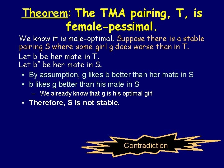
Theorem: The TMA pairing, T, is female-pessimal. We know it is male-optimal. Suppose there is a stable pairing S where some girl g does worse than in T. Let b be her mate in T. Let b* be her mate in S. • By assumption, g likes b better than her mate in S • b likes g better than his mate in S – We already know that g is his optimal girl • Therefore, S is not stable. Contradiction

Final Exam • Final Exam – – – Thursday 5/5 2 pm-5 Open book, open note Review session on Sunday in D 106 LSRC from 7: 45 pm -9 – Cumulative, Chapters 1 -9 • HW 1 -5 graded and posted • Submit any outstanding grading issues using assignment name issues Comp. Sci 102 18. 65