Today Alignment warping 2 d transformations Forward and

Today • Alignment & warping – 2 d transformations – Forward and inverse image warping – Constructing mosaics • Homographies • Robust fitting with RANSAC

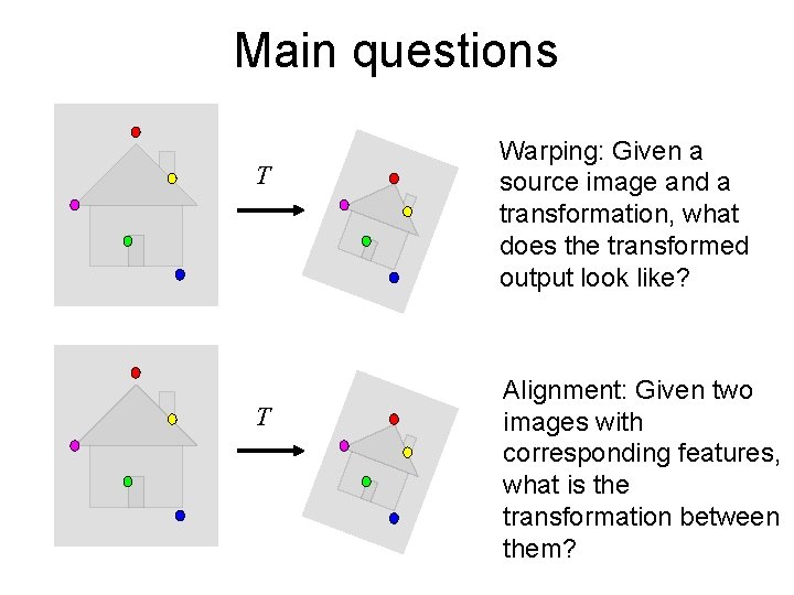
Main questions T T Warping: Given a source image and a transformation, what does the transformed output look like? Alignment: Given two images with corresponding features, what is the transformation between them?

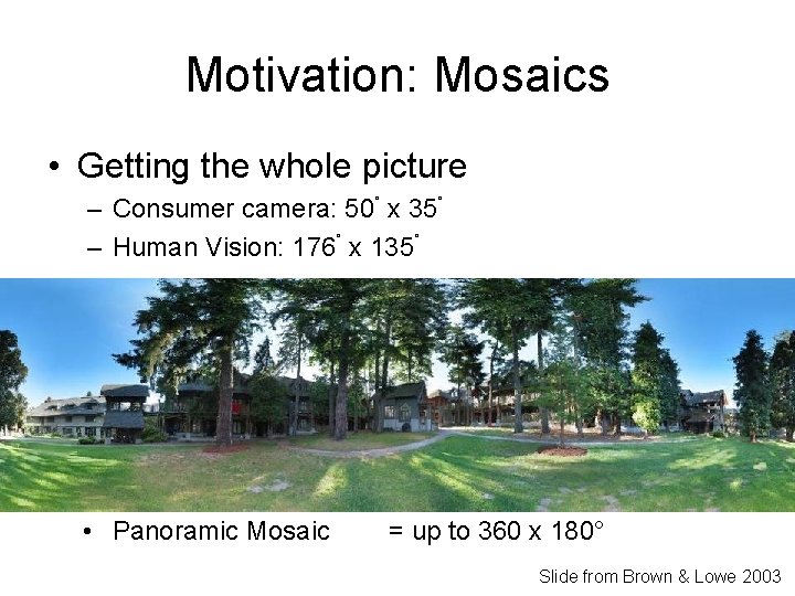
Motivation: Mosaics • Getting the whole picture – Consumer camera: 50˚ x 35˚ Slide from Brown & Lowe 2003

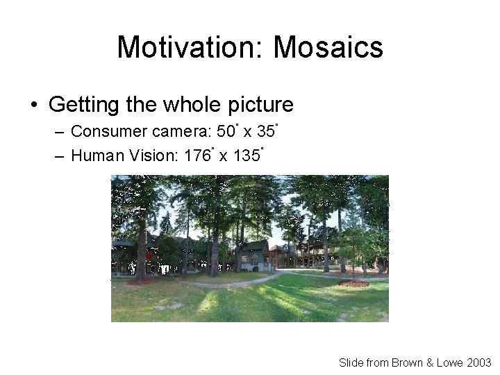
Motivation: Mosaics • Getting the whole picture – Consumer camera: 50˚ x 35˚ – Human Vision: 176˚ x 135˚ Slide from Brown & Lowe 2003

Motivation: Mosaics • Getting the whole picture – Consumer camera: 50˚ x 35˚ – Human Vision: 176˚ x 135˚ • Panoramic Mosaic = up to 360 x 180° Slide from Brown & Lowe 2003

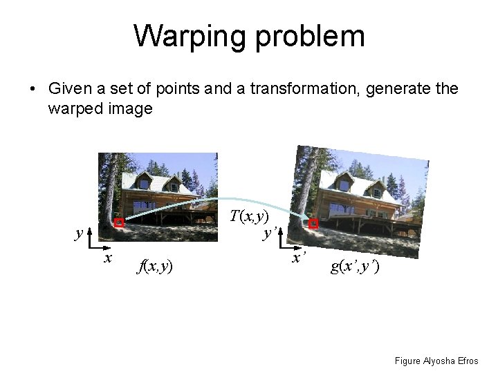
Warping problem • Given a set of points and a transformation, generate the warped image T(x, y) y’ y x f(x, y) x’ g(x’, y’) Figure Alyosha Efros

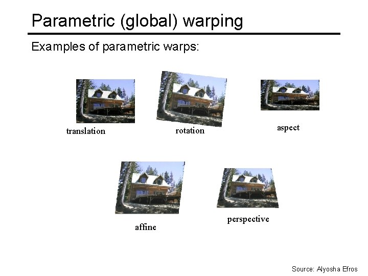
Parametric (global) warping Examples of parametric warps: aspect rotation translation affine perspective Source: Alyosha Efros

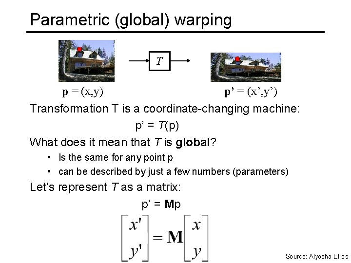
Parametric (global) warping T p = (x, y) p’ = (x’, y’) Transformation T is a coordinate-changing machine: p’ = T(p) What does it mean that T is global? • Is the same for any point p • can be described by just a few numbers (parameters) Let’s represent T as a matrix: p’ = Mp Source: Alyosha Efros

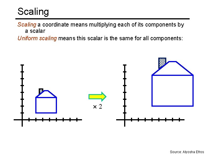
Scaling a coordinate means multiplying each of its components by a scalar Uniform scaling means this scalar is the same for all components: 2 Source: Alyosha Efros

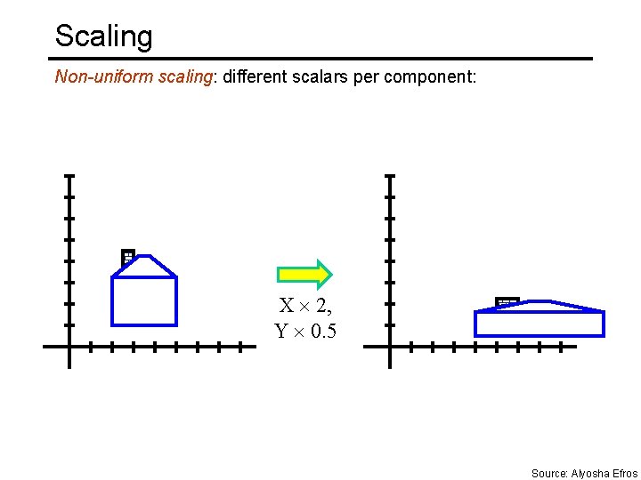
Scaling Non-uniform scaling: different scalars per component: X 2, Y 0. 5 Source: Alyosha Efros

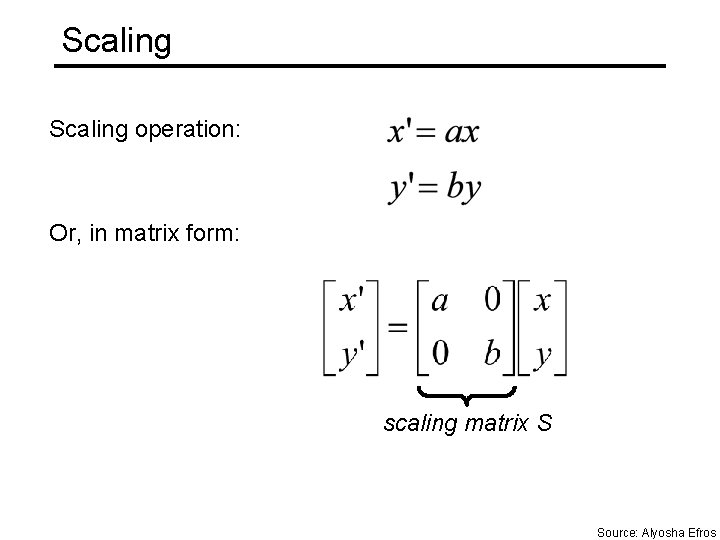
Scaling operation: Or, in matrix form: scaling matrix S Source: Alyosha Efros

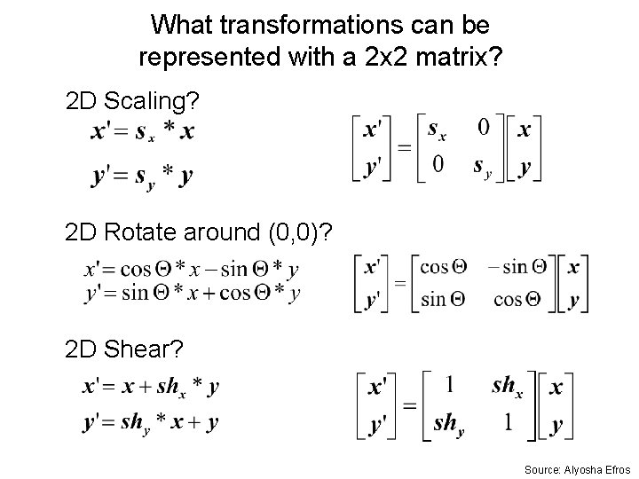
What transformations can be represented with a 2 x 2 matrix? 2 D Scaling? 2 D Rotate around (0, 0)? 2 D Shear? Source: Alyosha Efros

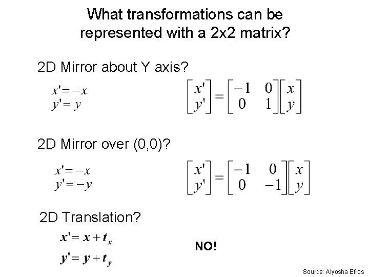
What transformations can be represented with a 2 x 2 matrix? 2 D Mirror about Y axis? 2 D Mirror over (0, 0)? 2 D Translation? NO! Source: Alyosha Efros

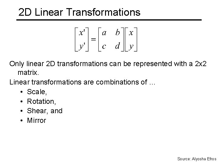
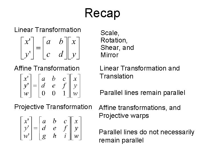
2 D Linear Transformations Only linear 2 D transformations can be represented with a 2 x 2 matrix. Linear transformations are combinations of … • Scale, • Rotation, • Shear, and • Mirror Source: Alyosha Efros

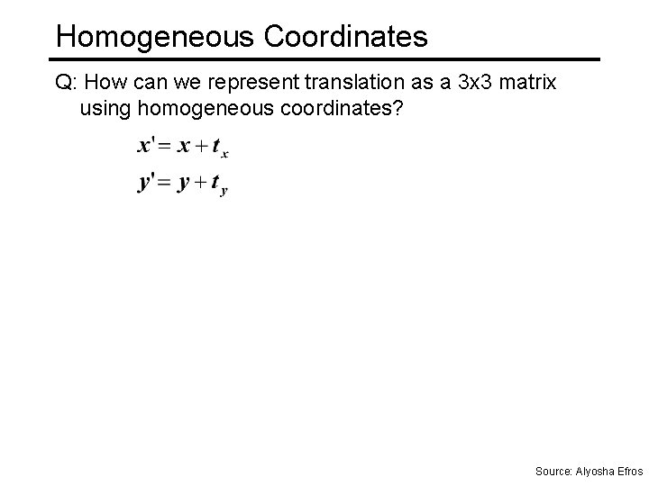
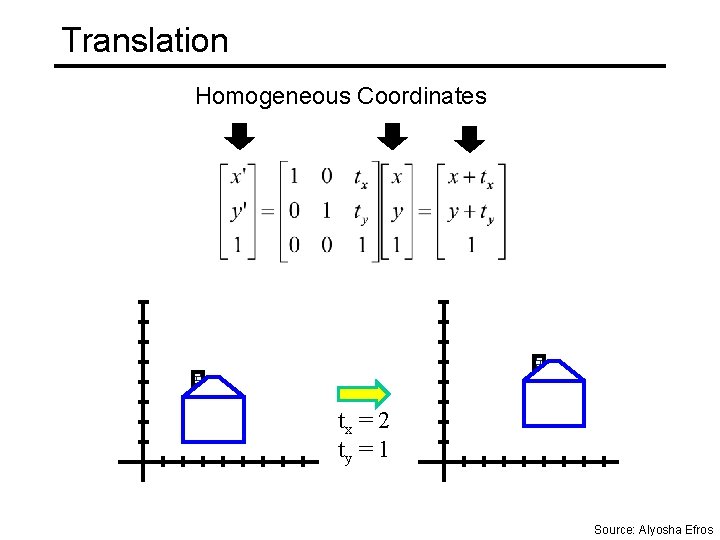
Homogeneous Coordinates Q: How can we represent translation as a 3 x 3 matrix using homogeneous coordinates? Source: Alyosha Efros

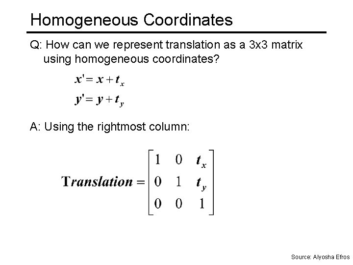
Homogeneous Coordinates Q: How can we represent translation as a 3 x 3 matrix using homogeneous coordinates? A: Using the rightmost column: Source: Alyosha Efros

Translation Homogeneous Coordinates tx = 2 ty = 1 Source: Alyosha Efros

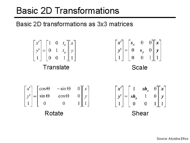
Basic 2 D Transformations Basic 2 D transformations as 3 x 3 matrices Translate Scale Rotate Shear Source: Alyosha Efros

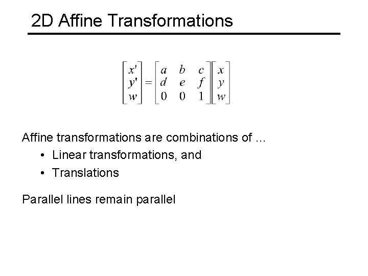
2 D Affine Transformations Affine transformations are combinations of … • Linear transformations, and • Translations Parallel lines remain parallel

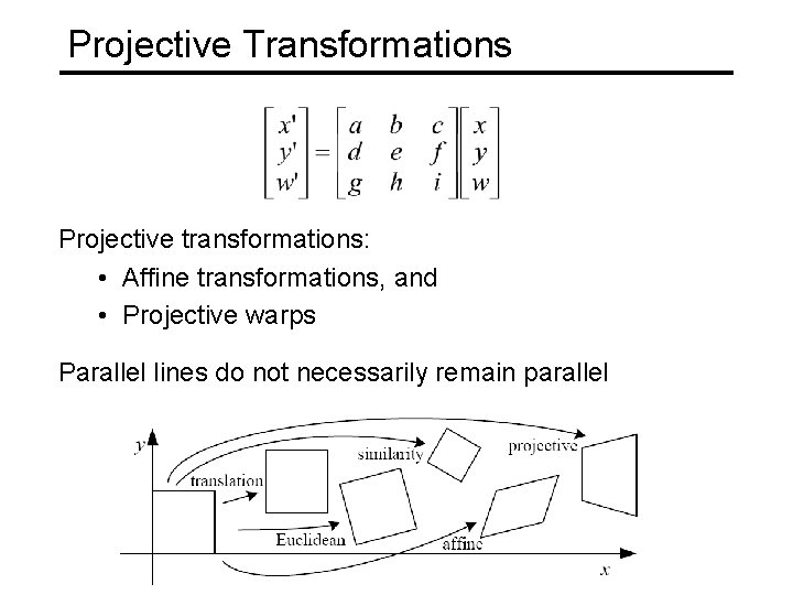
Projective Transformations Projective transformations: • Affine transformations, and • Projective warps Parallel lines do not necessarily remain parallel

Recap Linear Transformation Scale, Rotation, Shear, and Mirror Affine Transformation Linear Transformation and Translation Parallel lines remain parallel Projective Transformation Affine transformations, and Projective warps Parallel lines do not necessarily remain parallel

Today • Alignment & warping – 2 d transformations – Forward and inverse image warping – Constructing mosaics • Homographies • Robust fitting with RANSAC

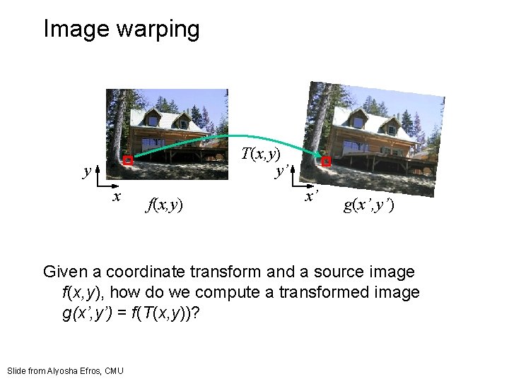
Image warping T(x, y) y’ y x f(x, y) x’ g(x’, y’) Given a coordinate transform and a source image f(x, y), how do we compute a transformed image g(x’, y’) = f(T(x, y))? Slide from Alyosha Efros, CMU

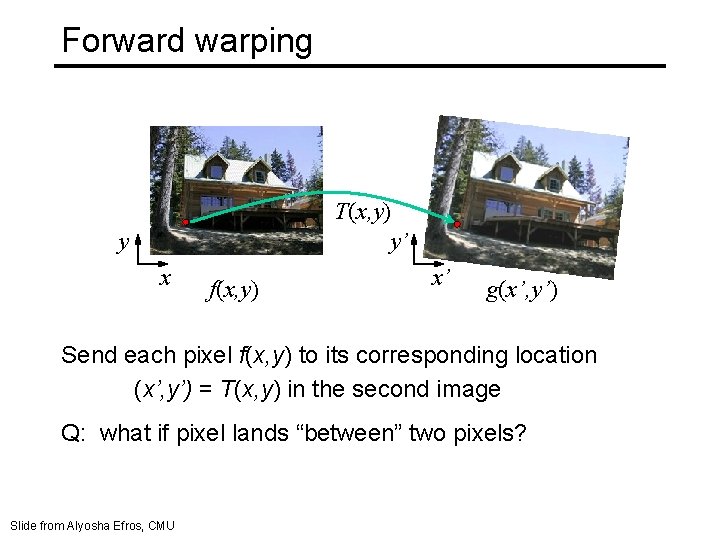
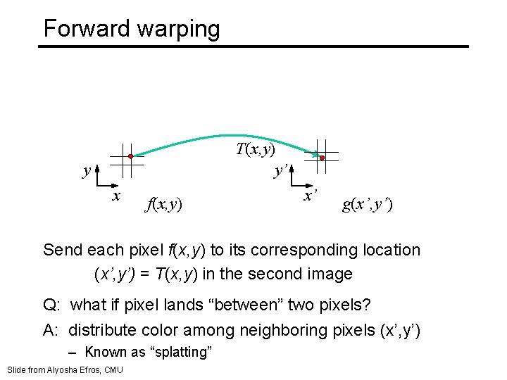
Forward warping T(x, y) y’ y x f(x, y) x’ g(x’, y’) Send each pixel f(x, y) to its corresponding location (x’, y’) = T(x, y) in the second image Q: what if pixel lands “between” two pixels? Slide from Alyosha Efros, CMU

Forward warping T(x, y) y’ y x f(x, y) x’ g(x’, y’) Send each pixel f(x, y) to its corresponding location (x’, y’) = T(x, y) in the second image Q: what if pixel lands “between” two pixels? A: distribute color among neighboring pixels (x’, y’) – Known as “splatting” Slide from Alyosha Efros, CMU

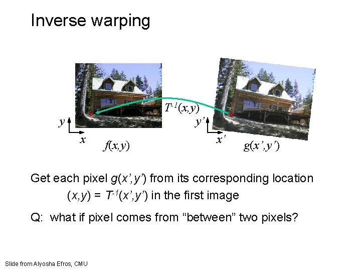
Inverse warping T-1(x, y) y’ y x f(x, y) x’ g(x’, y’) Get each pixel g(x’, y’) from its corresponding location (x, y) = T-1(x’, y’) in the first image Q: what if pixel comes from “between” two pixels? Slide from Alyosha Efros, CMU

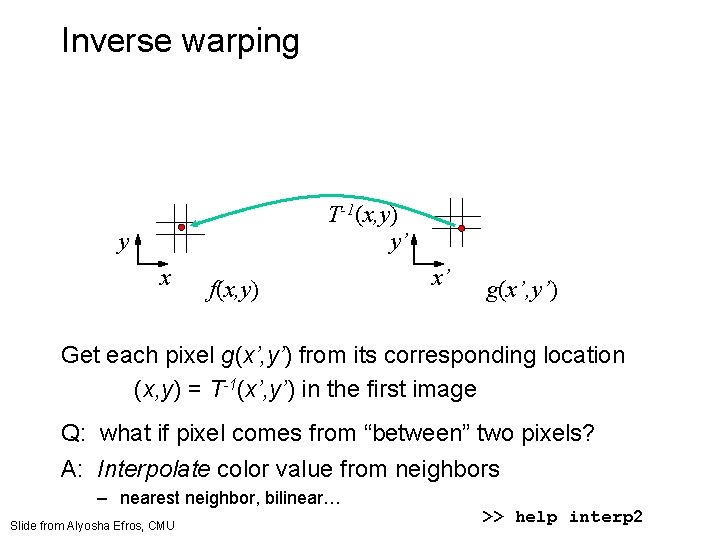
Inverse warping T-1(x, y) y’ y x f(x, y) x’ g(x’, y’) Get each pixel g(x’, y’) from its corresponding location (x, y) = T-1(x’, y’) in the first image Q: what if pixel comes from “between” two pixels? A: Interpolate color value from neighbors – nearest neighbor, bilinear… Slide from Alyosha Efros, CMU >> help interp 2

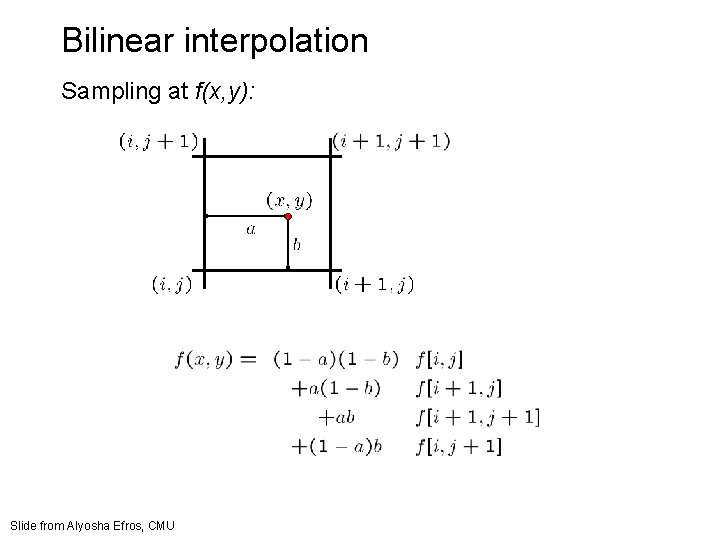
Bilinear interpolation Sampling at f(x, y): Slide from Alyosha Efros, CMU

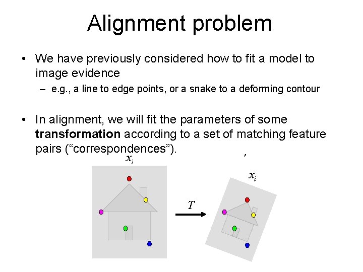
Alignment problem • We have previously considered how to fit a model to image evidence – e. g. , a line to edge points, or a snake to a deforming contour • In alignment, we will fit the parameters of some transformation according to a set of matching feature pairs (“correspondences”). ' xi xi T

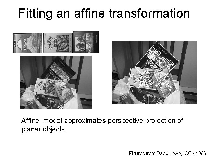
Fitting an affine transformation Affine model approximates perspective projection of planar objects. Figures from David Lowe, ICCV 1999

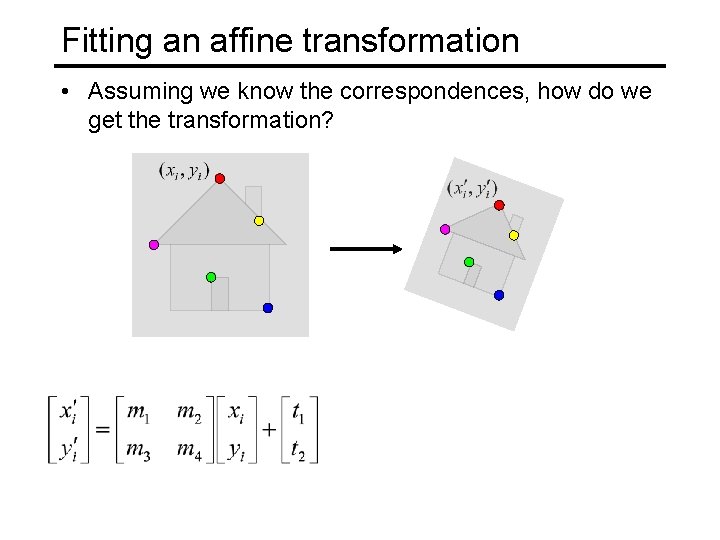
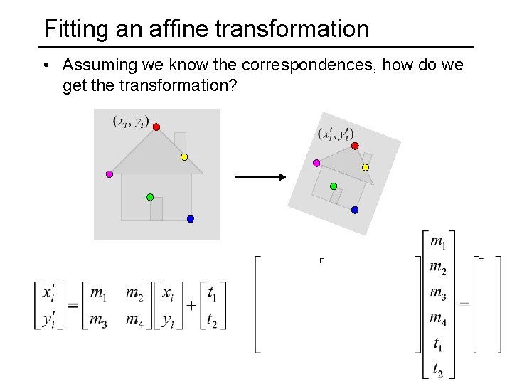
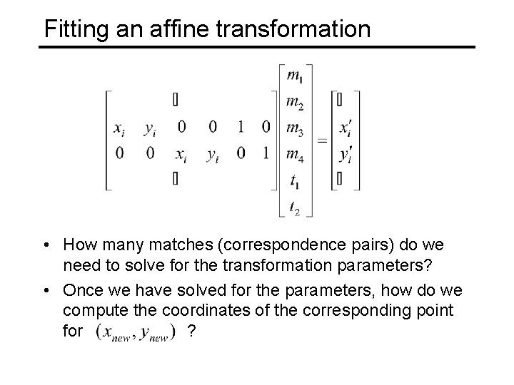
Fitting an affine transformation • Assuming we know the correspondences, how do we get the transformation?

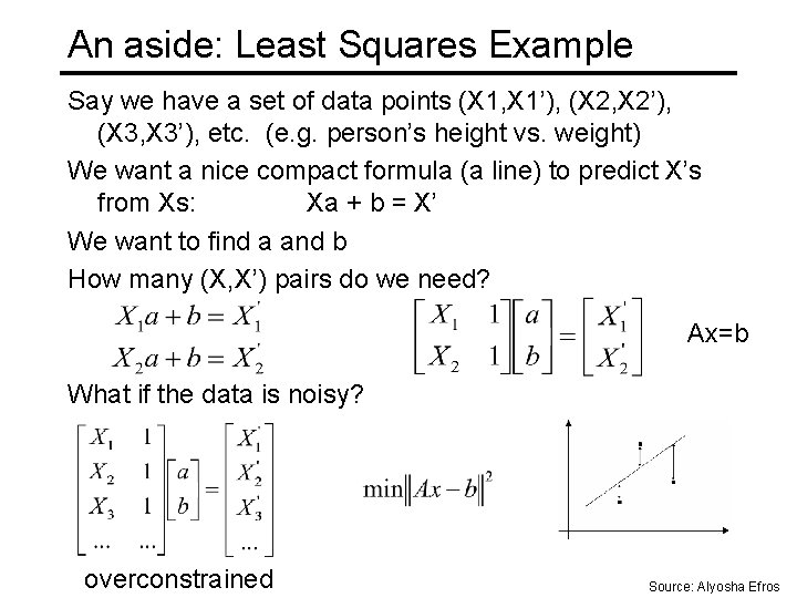
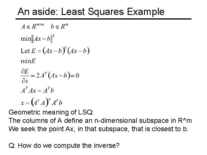
An aside: Least Squares Example Say we have a set of data points (X 1, X 1’), (X 2, X 2’), (X 3, X 3’), etc. (e. g. person’s height vs. weight) We want a nice compact formula (a line) to predict X’s from Xs: Xa + b = X’ We want to find a and b How many (X, X’) pairs do we need? Ax=b What if the data is noisy? overconstrained Source: Alyosha Efros

An aside: Least Squares Example Geometric meaning of LSQ: The columns of A define an n-dimensional subspace in R^m We seek the point Ax, in that subspace, that is closest to b. Q: How do we compute the inverse?

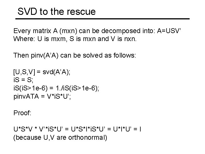
SVD to the rescue Every matrix A (mxn) can be decomposed into: A=USV’ Where: U is mxm, S is mxn and V is nxn. Then pinv(A’A) can be solved as follows: [U, S, V] = svd(A’A); i. S = S; i. S(i. S>1 e-6) = 1. /i. S(i. S>1 e-6); pinv. ATA = V*i. S*U’; Proof: U*S*V * V’*i. S*U’ = U*S*I*i. S*U’ = U*I*U’ = I (because U, V are orthonormal)

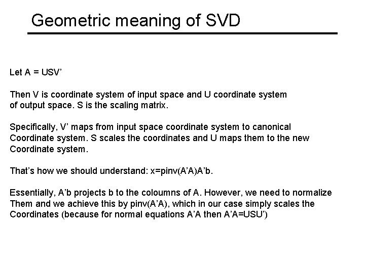
Geometric meaning of SVD Let A = USV’ Then V is coordinate system of input space and U coordinate system of output space. S is the scaling matrix. Specifically, V’ maps from input space coordinate system to canonical Coordinate system. S scales the coordinates and U maps them to the new Coordinate system. That’s how we should understand: x=pinv(A’A)A’b. Essentially, A’b projects b to the coloumns of A. However, we need to normalize Them and we achieve this by pinv(A’A), which in our case simply scales the Coordinates (because for normal equations A’A then A’A=USU’)

Fitting an affine transformation • Assuming we know the correspondences, how do we get the transformation?

Fitting an affine transformation • How many matches (correspondence pairs) do we need to solve for the transformation parameters? • Once we have solved for the parameters, how do we compute the coordinates of the corresponding point for ?

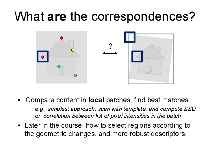
What are the correspondences? ? • Compare content in local patches, find best matches. e. g. , simplest approach: scan with template, and compute SSD or correlation between list of pixel intensities in the patch • Later in the course: how to select regions according to the geometric changes, and more robust descriptors.

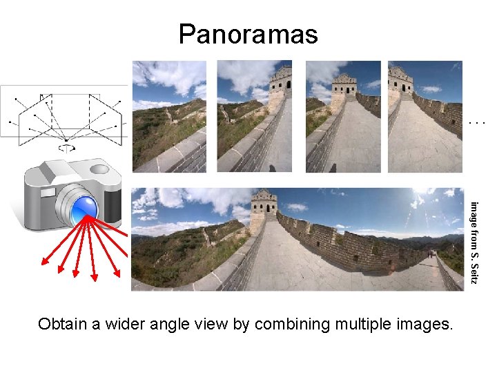
Panoramas. . . image from S. Seitz Obtain a wider angle view by combining multiple images.

How to stitch together a panorama? • Basic Procedure – Take a sequence of images from the same position • Rotate the camera about its optical center – Compute transformation between second image and first – Transform the second image to overlap with the first – Blend the two together to create a mosaic – (If there are more images, repeat) • …but wait, why should this work at all? – What about the 3 D geometry of the scene? – Why aren’t we using it? Source: Steve Seitz

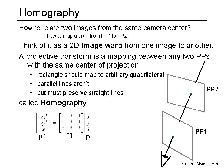
Homography How to relate two images from the same camera center? – how to map a pixel from PP 1 to PP 2? Think of it as a 2 D image warp from one image to another. A projective transform is a mapping between any two PPs with the same center of projection • rectangle should map to arbitrary quadrilateral • parallel lines aren’t • but must preserve straight lines PP 2 called Homography p’ H p PP 1 Source: Alyosha Efros

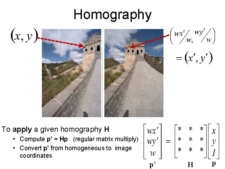
Homography To apply a given homography H • Compute p’ = Hp (regular matrix multiply) • Convert p’ from homogeneous to image coordinates p’ H p

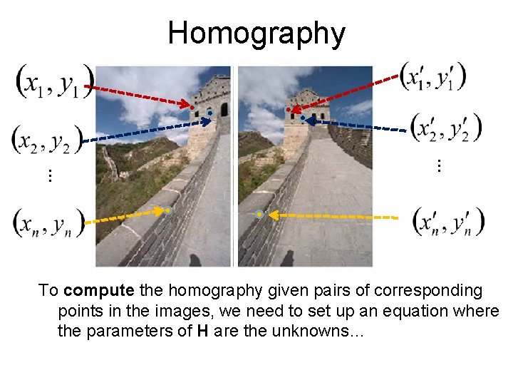
Homography … … To compute the homography given pairs of corresponding points in the images, we need to set up an equation where the parameters of H are the unknowns…

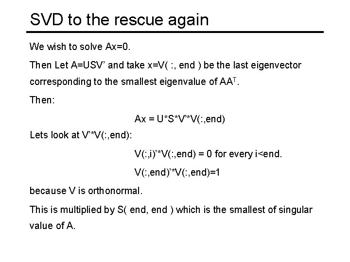
SVD to the rescue again We wish to solve Ax=0. Then Let A=USV’ and take x=V( : , end ) be the last eigenvector corresponding to the smallest eigenvalue of AAT. Then: Ax = U*S*V’*V(: , end) Lets look at V’*V(: , end): V(: , i)’*V(: , end) = 0 for every i<end. V(: , end)’*V(: , end)=1 because V is orthonormal. This is multiplied by S( end, end ) which is the smallest of singular value of A.

Recap: How to stitch together a panorama? • Basic Procedure – Take a sequence of images from the same position • Rotate the camera about its optical center – Compute transformation between second image and first – Transform the second image to overlap with the first – Blend the two together to create a mosaic – (If there are more images, repeat) Source: Steve Seitz

Today • Alignment & warping – 2 d transformations – Forward and inverse image warping – Constructing mosaics • Homographies • Robust fitting with RANSAC

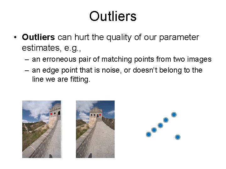
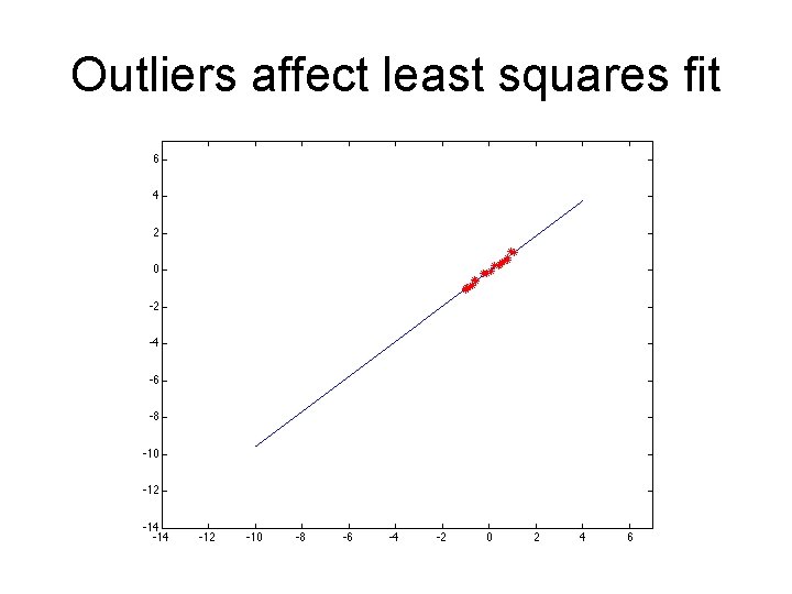
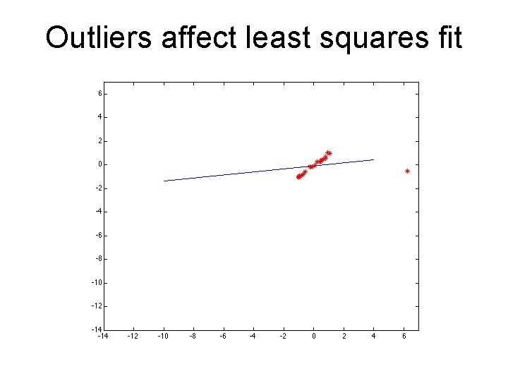
Outliers • Outliers can hurt the quality of our parameter estimates, e. g. , – an erroneous pair of matching points from two images – an edge point that is noise, or doesn’t belong to the line we are fitting.

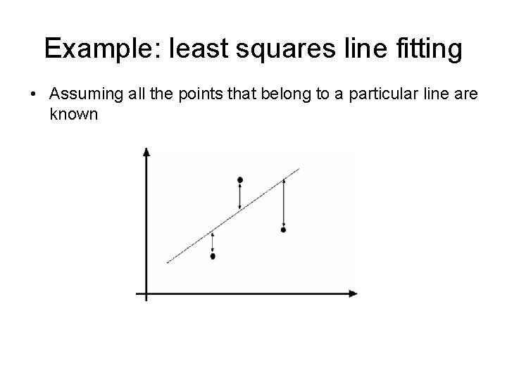
Example: least squares line fitting • Assuming all the points that belong to a particular line are known

Outliers affect least squares fit

Outliers affect least squares fit

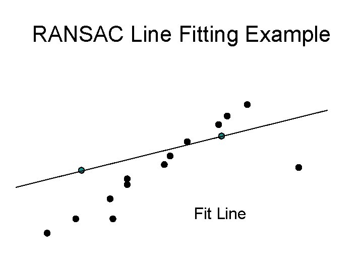
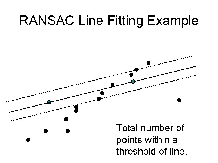
RANSAC • RANdom Sample Consensus • Approach: we want to avoid the impact of outliers, so let’s look for “inliers”, and use those only. • Intuition: if an outlier is chosen to compute the current fit, then the resulting line won’t have much support from rest of the points.

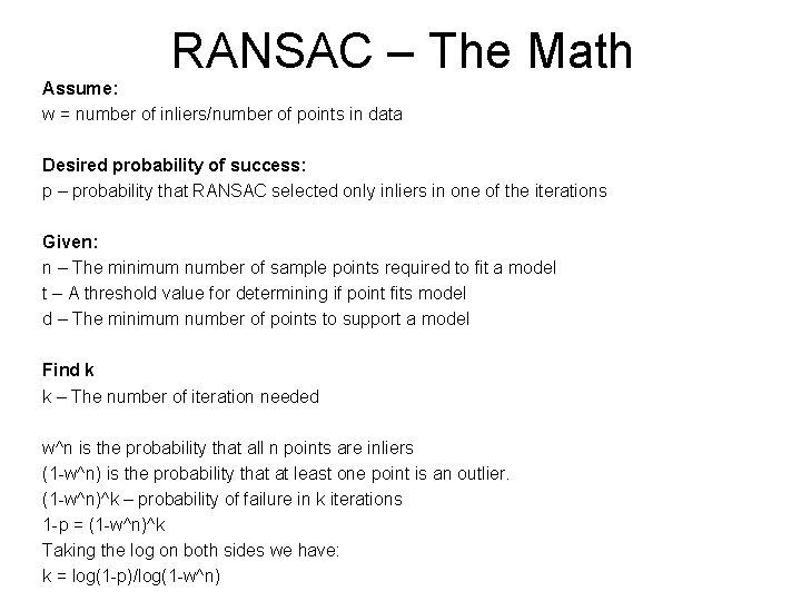
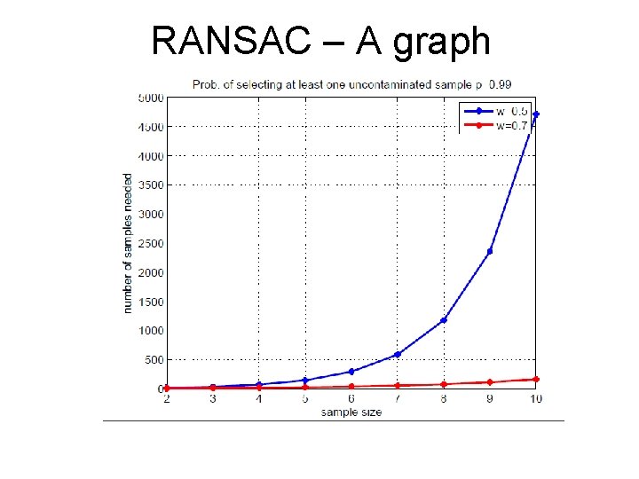
RANSAC – The Math Assume: w = number of inliers/number of points in data Desired probability of success: p – probability that RANSAC selected only inliers in one of the iterations Given: n – The minimum number of sample points required to fit a model t – A threshold value for determining if point fits model d – The minimum number of points to support a model Find k k – The number of iteration needed w^n is the probability that all n points are inliers (1 -w^n) is the probability that at least one point is an outlier. (1 -w^n)^k – probability of failure in k iterations 1 -p = (1 -w^n)^k Taking the log on both sides we have: k = log(1 -p)/log(1 -w^n)

RANSAC – A graph

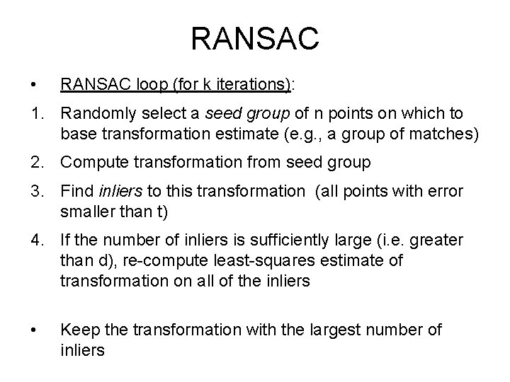
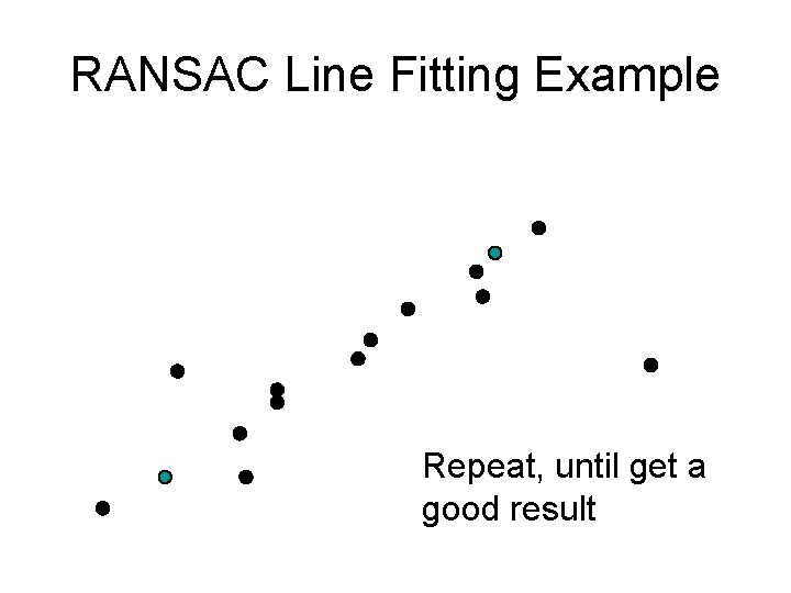
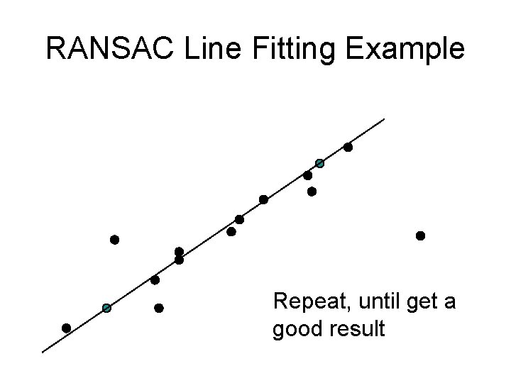
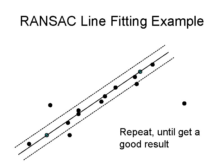
RANSAC • RANSAC loop (for k iterations): 1. Randomly select a seed group of n points on which to base transformation estimate (e. g. , a group of matches) 2. Compute transformation from seed group 3. Find inliers to this transformation (all points with error smaller than t) 4. If the number of inliers is sufficiently large (i. e. greater than d), re-compute least-squares estimate of transformation on all of the inliers • Keep the transformation with the largest number of inliers

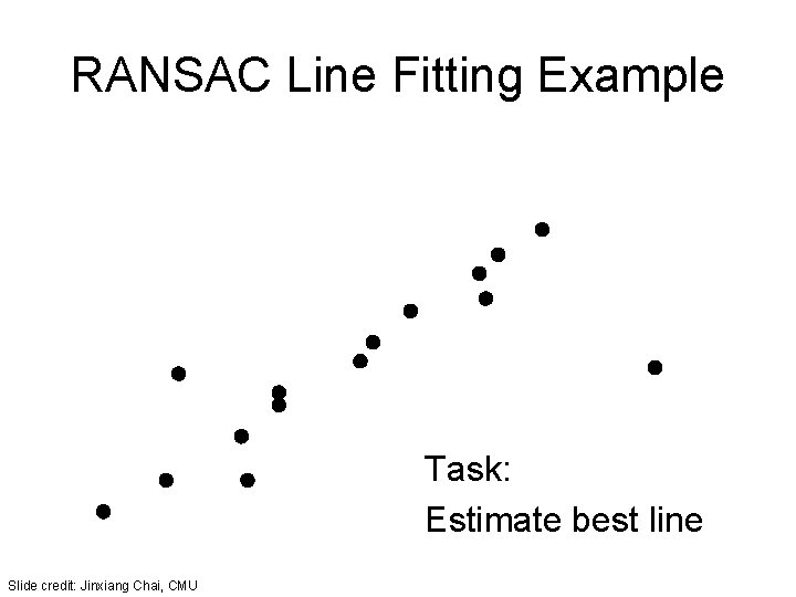
RANSAC Line Fitting Example Task: Estimate best line Slide credit: Jinxiang Chai, CMU

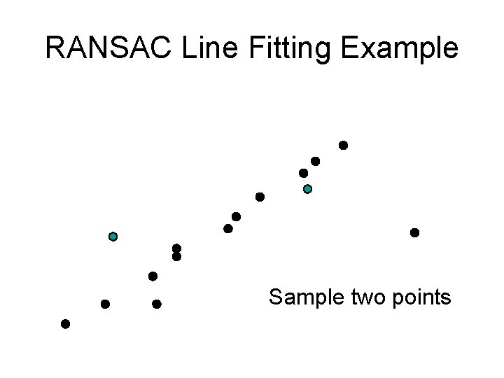
RANSAC Line Fitting Example Sample two points

RANSAC Line Fitting Example Fit Line

RANSAC Line Fitting Example Total number of points within a threshold of line.

RANSAC Line Fitting Example Repeat, until get a good result

RANSAC Line Fitting Example Repeat, until get a good result

RANSAC Line Fitting Example Repeat, until get a good result

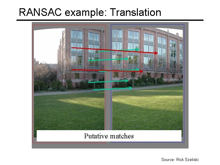
RANSAC example: Translation Putative matches Source: Rick Szeliski

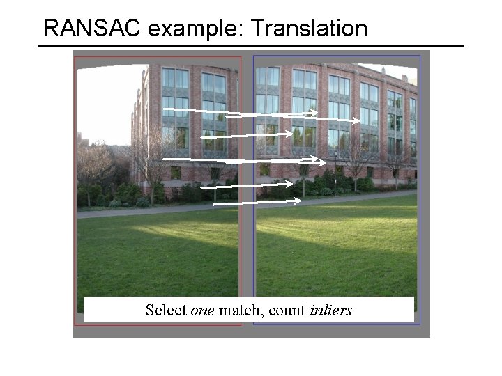
RANSAC example: Translation Select one match, count inliers

RANSAC example: Translation Select one match, count inliers

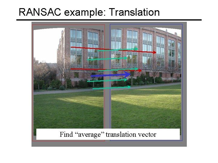
RANSAC example: Translation Find “average” translation vector

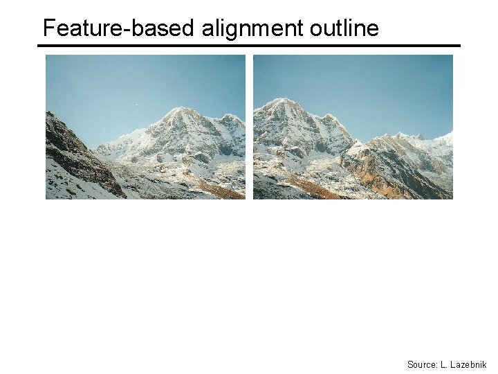
Feature-based alignment outline Source: L. Lazebnik

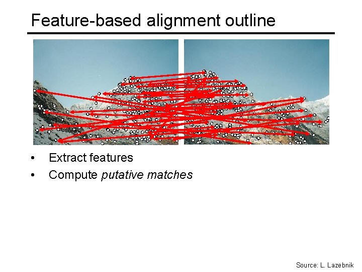
Feature-based alignment outline • Extract features Source: L. Lazebnik

Feature-based alignment outline • • Extract features Compute putative matches Source: L. Lazebnik

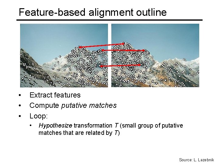
Feature-based alignment outline • • • Extract features Compute putative matches Loop: • Hypothesize transformation T (small group of putative matches that are related by T) Source: L. Lazebnik

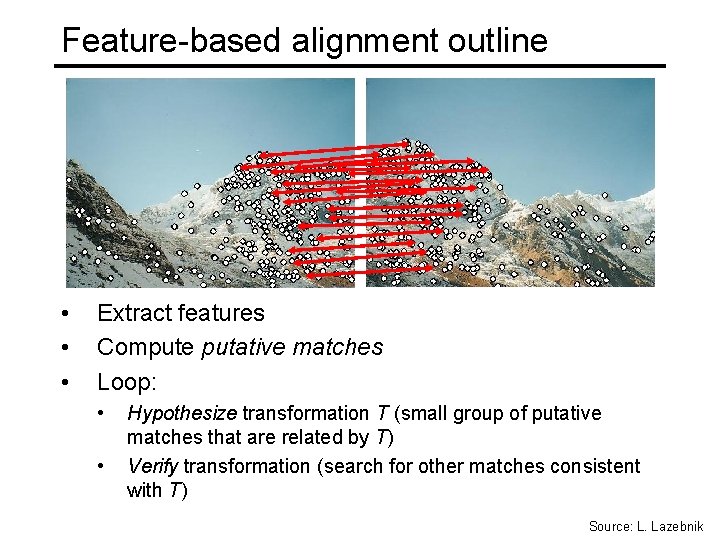
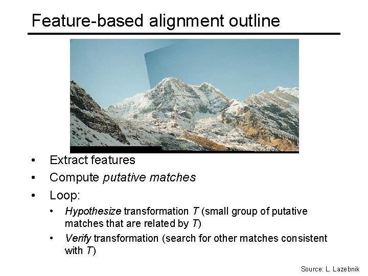
Feature-based alignment outline • • • Extract features Compute putative matches Loop: • • Hypothesize transformation T (small group of putative matches that are related by T) Verify transformation (search for other matches consistent with T) Source: L. Lazebnik

Feature-based alignment outline • • • Extract features Compute putative matches Loop: • • Hypothesize transformation T (small group of putative matches that are related by T) Verify transformation (search for other matches consistent with T) Source: L. Lazebnik

Today • Alignment & warping – 2 d transformations – Forward and inverse image warping – Constructing mosaics • Homographies • Robust fitting with RANSAC