Introduction to Digital Signal Processing DSP Part 4

Introduction to Digital Signal Processing (DSP) Part 4 of 4 (“Typical GN&C Applications”) James R. (Jim) Beaty, Ph. D - NASA Langley Research Center Vehicle Analysis Branch, Systems Analysis & Concepts Directorate Bldg 1209, Room 128 B, M/S 451 1 North Dryden Street Hampton, VA 23681 757 -864 -1322 James. R. Beaty@nasa. gov Learning from the Past, Looking to the Future Page: 1

Overview • Part 1, “Mathematical Concepts” – Definitions, mathematical pre-requisites, and application techniques • Fourier transforms and convolution • Discrete Fourier transforms (DFT) and Fast Fourier transforms (FFT) • Shannon Sampling Theorem and data aliasing • Part 2, “Power Spectral Density Basics” – Power Spectral Density (PSD) to estimate spectral characteristics of waveforms – PSD Demonstration • Part 3 “Implementing Discrete Filters” – Converting from continuous Laplace domain filters to discrete Z-domain filters (Tustin’s rule, or bilinear transformation) – Recursive filter implementations for discrete filters • Part 4 “Typical GN&C Applications” – – – Normalized frequency Methods to verify transfer function magnitude/phase of discrete filters using DFT (or FFT) Example use of discrete filter to implement a notch filter Learning from the Past, Looking to the Future Page: 2

Normalized Frequency • • One of the most confusing concepts of digital signal processing in general, and DFTs / FFTs in particular, is the concept of normalized frequency A Laplace domain filter specifies the filter response in terms of a natural frequency (also known as “corner” frequency) – usually in units of radians/second, if w, or wn is used to denote the filter frequency – sometimes in hertz (cycles/second), if f or fn is used to denote the filter frequency • • When Laplace domain filters are converted to discrete filters, the calculations for the discrete filter coefficients contain terms like “w. T/2” The discrete filter is entirely described by the normalized frequency, which is the ratio of the “natural frequency” of the filter (in hertz) divided by the update frequency (in hertz), of the discrete filter: – f. S (the sample frequency in hertz) = 1 / ( T, seconds per sample ) – Now, since T = 1 / f. S, then w. T/2 = 2 pf /f. S /2, = p (f/ f. S), and ( f / f. S ) = the normalized frequency • So, “w. T/2” shown in the equations which define the filter coefficients can be replaced with normalized frequency multiplied by p Learning from the Past, Looking to the Future Page: 3

Normalized Frequency - Continued • • When a DFT (or FFT) is computed for an input sequence, the output frequency is normalized to the sample frequency, (f / f. S) – For entirely real sequences, the range of normalized frequencies is 0 to 0. 5 – For complex sequences, the range of normalized frequencies is ± 0. 5 – A normalized frequency of 0. 5 represents the Nyquist frequency, or half the sample frequency – A discrete filter cannot implement frequencies above the Nyquist frequency To convert the normalized frequency computed by the DFT (or FFT) of a signal into “real” frequency (e. g. – hertz, or radians/second), the output normalized frequency must be multiplied by the sample frequency, f. S = 1/T, (for output in hertz), or 2 p times the sample frequency (for output in radians per second) Learning from the Past, Looking to the Future Page: 4

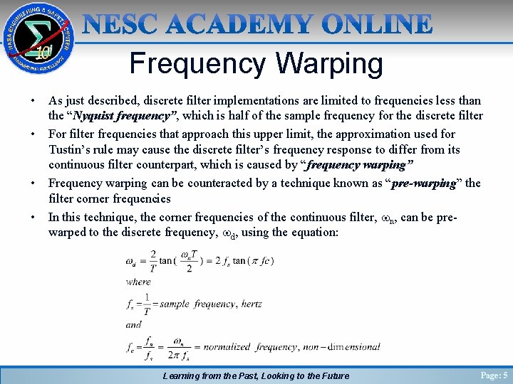
Frequency Warping • • As just described, discrete filter implementations are limited to frequencies less than the “Nyquist frequency”, which is half of the sample frequency for the discrete filter For filter frequencies that approach this upper limit, the approximation used for Tustin’s rule may cause the discrete filter’s frequency response to differ from its continuous filter counterpart, which is caused by “frequency warping” Frequency warping can be counteracted by a technique known as “pre-warping” the filter corner frequencies In this technique, the corner frequencies of the continuous filter, wn, can be prewarped to the discrete frequency, wd, using the equation: Learning from the Past, Looking to the Future Page: 5

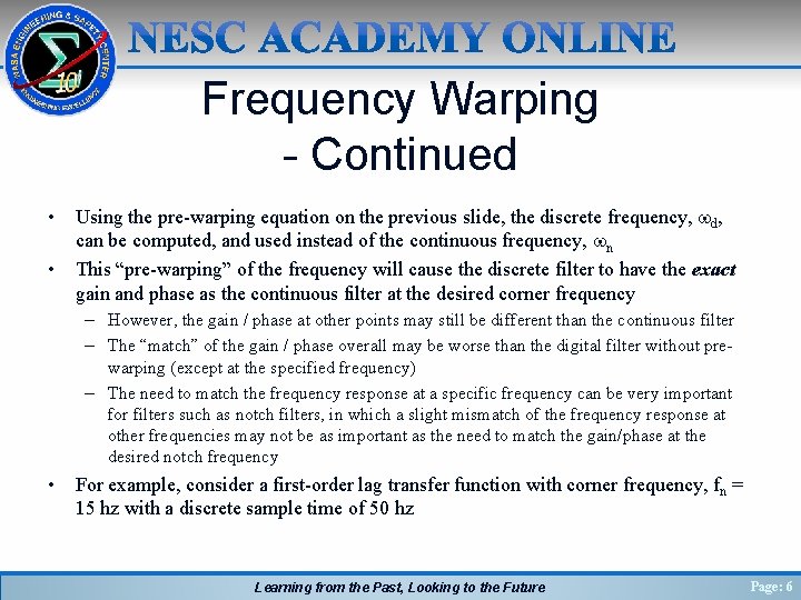
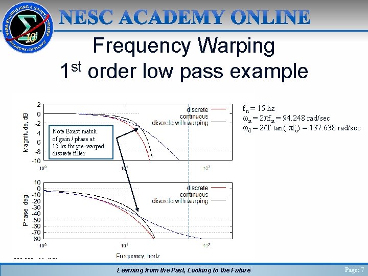
Frequency Warping - Continued • • Using the pre-warping equation on the previous slide, the discrete frequency, wd, can be computed, and used instead of the continuous frequency, wn This “pre-warping” of the frequency will cause the discrete filter to have the exact gain and phase as the continuous filter at the desired corner frequency – However, the gain / phase at other points may still be different than the continuous filter – The “match” of the gain / phase overall may be worse than the digital filter without prewarping (except at the specified frequency) – The need to match the frequency response at a specific frequency can be very important for filters such as notch filters, in which a slight mismatch of the frequency response at other frequencies may not be as important as the need to match the gain/phase at the desired notch frequency • For example, consider a first-order lag transfer function with corner frequency, fn = 15 hz with a discrete sample time of 50 hz Learning from the Past, Looking to the Future Page: 6

Frequency Warping 1 st order low pass example Note Exact match of gain / phase at 15 hz for pre-warped discrete filter fn = 15 hz wn = 2 pfn = 94. 248 rad/sec wd = 2/T tan( pfc) = 137. 638 rad/sec Learning from the Past, Looking to the Future Page: 7

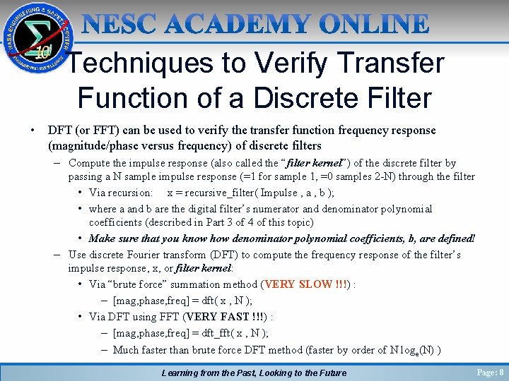
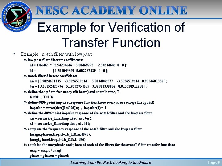
Techniques to Verify Transfer Function of a Discrete Filter • DFT (or FFT) can be used to verify the transfer function frequency response (magnitude/phase versus frequency) of discrete filters – Compute the impulse response (also called the “filter kernel”) of the discrete filter by passing a N sample impulse response (=1 for sample 1, =0 samples 2 -N) through the filter • Via recursion: x = recursive_filter( Impulse , a , b ); • where a and b are the digital filter’s numerator and denominator polynomial coefficients (described in Part 3 of 4 of this topic) • Make sure that you know how denominator polynomial coefficients, b, are defined! – Use discrete Fourier transform (DFT) to compute the frequency response of the filter’s impulse response, x, or filter kernel: • Via “brute force” summation method (VERY SLOW !!!) : – [mag, phase, freq] = dft( x , N ); • Via DFT using FFT (VERY FAST !!!) : – [mag, phase, freq] = dft_fft( x , N ); – Much faster than brute force DFT method (faster by order of N loge(N) ) Learning from the Past, Looking to the Future Page: 8

Example for Verification of Transfer Function • Example: notch filter with lowpass: % low pass filter discrete coefficients: al = 1. 0 e-02 * [ 2. 54234646 5. 08469292 2. 54234646 0 0 ]; bl = [ 1. 501043369 -0. 602737225 0 0 ]; % notch filter discrete coefficients: an = [ 0. 9024681335 -3. 5026519614 5. 2034846577 -3. 5026519614 0. 9024681336 ]; bn = [ 3. 68352427976 -5. 19672754635 3. 32581338106 -0. 815728911280 ]; % define the update frequency (50 hertz) and sample time, T fs=50; , T=1/fs; % define 4096 point impulse response function (zero everywhere except first point) impulse = zeros(size([1: 4096])); , impulse(1) = 1; % define the 4096 point impulse response of the notch filter and the lowpass filter xn = recursive_filter(impulse , an , bn ); xl = recursive_filter(impulse , al , bl ); % compute the frequency response of the notch filter and the lowpass filter [magn, phasen, freqn]=dft_fft(xn, 4096); [magl, phasel, freql]=dft_fft(xl, 4096); % combine the magnitude and phase of each of the filters for the overall filter transfer function: mag = magn + magl; phase = phasen + phasel; Learning from the Past, Looking to the Future Page: 9

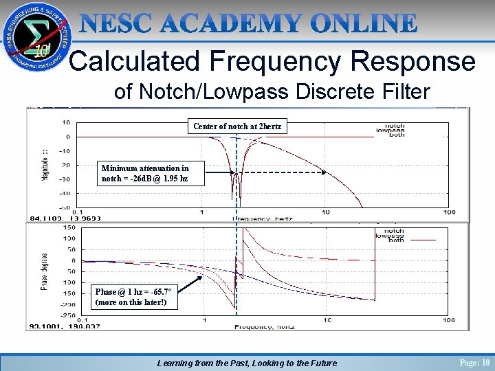
Calculated Frequency Response of Notch/Lowpass Discrete Filter Center of notch at 2 hertz Minimum attenuation in notch = -26 d. B @ 1. 95 hz Phase @ 1 hz = -65. 7° (more on this later!) Learning from the Past, Looking to the Future Page: 10

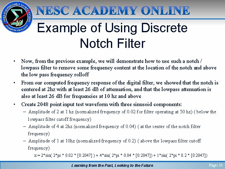
Example of Using Discrete Notch Filter • • • Now, from the previous example, we will demonstrate how to use such a notch / lowpass filter to remove some frequency content at the location of the notch and above the low pass frequency rolloff From our computed frequency response of the digital filter, we showed that the notch is centered at 2 hz with at least 26 d. B of attenuation, and that the lowpass attenuation is also at least 26 d. B for frequencies at 10 hz and above Create 2048 point input test waveform with three sinusoid components: – Amplitude of 2 at 1 hz (normalized frequency of 0. 02 for filter operating at 50 hz) ( below the lowpass filter cutoff frequency) – Amplitude of 4 at 2 hz (normalized frequency of 0. 04) ( at the center of the notch filter frequency) – Amplitude of 1 at 10 hz (normalized frequency of 0. 2) ( above the lowpass filter cutoff frequency) x = 2*sin( 2*pi * 0. 02 * [0: 2047] ) + 4*sin( 2*pi * 0. 04 * [0: 2047]) + 1*sin( 2*pi * 0. 2 * [0: 2047]) Learning from the Past, Looking to the Future Page: 11

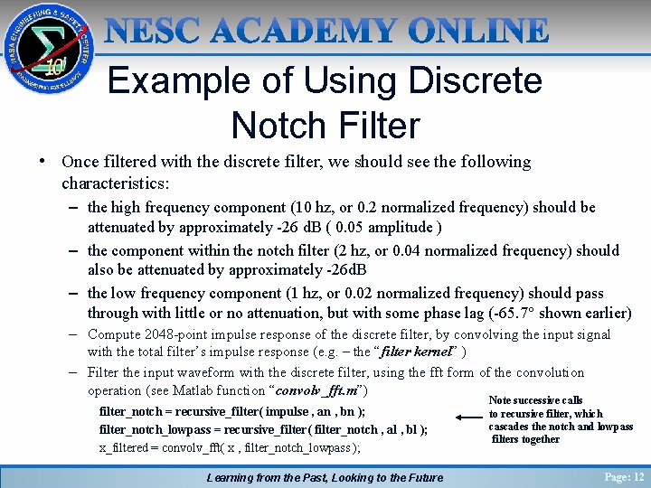
Example of Using Discrete Notch Filter • Once filtered with the discrete filter, we should see the following characteristics: – the high frequency component (10 hz, or 0. 2 normalized frequency) should be attenuated by approximately -26 d. B ( 0. 05 amplitude ) – the component within the notch filter (2 hz, or 0. 04 normalized frequency) should also be attenuated by approximately -26 d. B – the low frequency component (1 hz, or 0. 02 normalized frequency) should pass through with little or no attenuation, but with some phase lag (-65. 7° shown earlier) – Compute 2048 -point impulse response of the discrete filter, by convolving the input signal with the total filter’s impulse response (e. g. – the “filter kernel” ) – Filter the input waveform with the discrete filter, using the fft form of the convolution operation (see Matlab function “convolv_fft. m”) filter_notch = recursive_filter( impulse , an , bn ); filter_notch_lowpass = recursive_filter( filter_notch , al , bl ); x_filtered = convolv_fft( x , filter_notch_lowpass ); Learning from the Past, Looking to the Future Note successive calls to recursive filter, which cascades the notch and lowpass filters together Page: 12

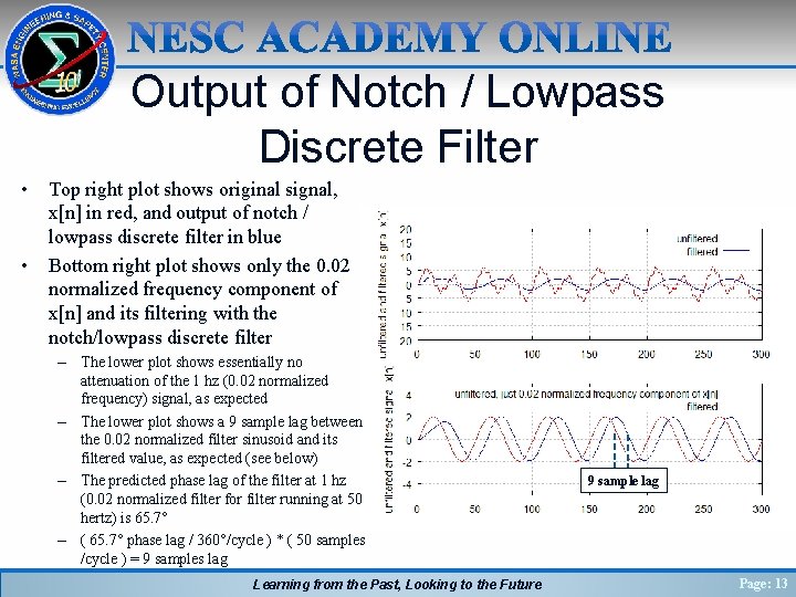
Output of Notch / Lowpass Discrete Filter • • Top right plot shows original signal, x[n] in red, and output of notch / lowpass discrete filter in blue Bottom right plot shows only the 0. 02 normalized frequency component of x[n] and its filtering with the notch/lowpass discrete filter – The lower plot shows essentially no attenuation of the 1 hz (0. 02 normalized frequency) signal, as expected – The lower plot shows a 9 sample lag between the 0. 02 normalized filter sinusoid and its filtered value, as expected (see below) – The predicted phase lag of the filter at 1 hz (0. 02 normalized filter for filter running at 50 hertz) is 65. 7° – ( 65. 7° phase lag / 360°/cycle ) * ( 50 samples /cycle ) = 9 samples lag Learning from the Past, Looking to the Future 9 sample lag Page: 13

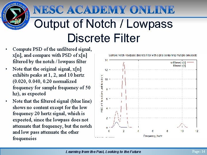
Output of Notch / Lowpass Discrete Filter • • • Compute PSD of the unfiltered signal, x[n], and compare with PSD of x[n] filtered by the notch / lowpass filter Note that the original signal, x[n] exhibits peaks at 1, 2, and 10 hertz (0. 020, 0. 040, 0. 20 normalized frequency for sample frequency of 50 hz), as expected Note that the filtered signal (blue line) shows no content except for the low frequency 20 hertz signal, which is expected, since the lowpass does not attenuate that frequency, but the notch and low pass attenuate the other frequencies Learning from the Past, Looking to the Future Page: 14

Frequency Response of original signal, x[n] and filtered signal • • Compute 1024 point DFT of the unfiltered signal, x[n], and compare magnitude with that of x[n] filtered by the notch / lowpass filter Note very little attenuation in magnitude at low frequency (1 hz), as expected Note that the sharp attenuation at the 2 hz notch location of >26 d. B, as expected Note the wider region of attenuation for the higher frequencies above 2 hz, with >26 d. B at 10 hertz, as expected Learning from the Past, Looking to the Future Page: 15

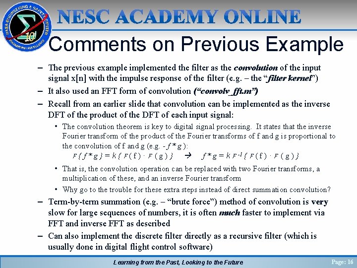
Comments on Previous Example – The previous example implemented the filter as the convolution of the input signal x[n] with the impulse response of the filter (e. g. – the “filter kernel”) – It also used an FFT form of convolution (“convolv_fft. m”) – Recall from an earlier slide that convolution can be implemented as the inverse DFT of the product of the DFT of each input signal: • The convolution theorem is key to digital signal processing. It states that the inverse Fourier transform of the product of the Fourier transforms of f and g is proportional to the convolution of f and g (e. g. - f * g ): F { f * g } = k { F ( f ) · F ( g ) } f * g = k F -1 { F ( f ) · F ( g ) } • That is, the convolution operation can be replaced with two Fourier transforms, a multiplication of these, and an inverse Fourier transform • Why go to the trouble for these extra steps instead of direct summation convolution? – Term-by-term summation (e. g. – “brute force”) method of convolution is very slow for large sequences of numbers, it is often much faster to implement via FFT and inverse FFT as described – Can also implement the discrete filter directly as a recursive filter (which is usually done in digital flight control software) Learning from the Past, Looking to the Future Page: 16

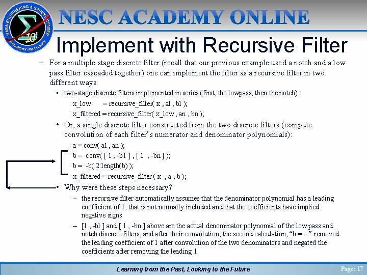
Implement with Recursive Filter – For a multiple stage discrete filter (recall that our previous example used a notch and a low pass filter cascaded together) one can implement the filter as a recursive filter in two different ways: • two-stage discrete filters implemented in series (first, the lowpass, then the notch) : x_low = recursive_filter( x , al , bl ); x_filtered = recursive_filter( x_low , an , bn ); • Or, a single discrete filter constructed from the two discrete filters (compute convolution of each filter’s numerator and denominator polynomials): a = conv( al , an ); b = conv( [ 1 , -b 1 ] , [ 1 , -bn ] ); b = -b( 2: length(b) ); x_filtered = recursive_filter ( x , a , b ); • Why were these steps necessary? – the recursive filter automatically assumes that the denominator polynomial has a leading coefficient of 1, that is not normally included and that the coefficients have implied negative signs – [1 , -bl ] and [ 1 , -bn ] above are the actual denominator polynomial of the low pass and notch discrete filters, and after their convolution, the second calculation, “b =. . . ” removed the leading coefficient of 1 after convolution of the two denominators and negated the coefficients after removing the leading 1 Learning from the Past, Looking to the Future Page: 17

Introduction to DSP, Part 4 of 4 Summary • In Part 1, “Mathematical Concepts” we covered the following: – Definitions, mathematical pre-requisites, and application techniques • Fourier transforms and convolution • Discrete Fourier transforms (DFT) and Fast Fourier transforms (FFT) • Shannon Sampling Theorem and data aliasing • In Part 2, “Power Spectral Density Basics”, we covered the following: – Power Spectral Density (PSD) to estimate spectral characteristics of waveforms – PSD Demonstration • In Part 3 “Implementing Discrete Filters” we covered the following: – Converting from continuous Laplace domain filters to discrete Z-domain filters (Tustin’s rule, or bilinear transformation) – Recursive filter implementations for discrete filters • In Part 4 “Typical GN&C Applications” we have covered the following: – – – Normalized frequency Methods to verify transfer function magnitude/phase of discrete filters using DFT (or FFT) Example use of discrete filter to implement a notch filter Learning from the Past, Looking to the Future Page: 18