Time Series Econometrics Lecture 3 ARMA Models Cont

Time Series Econometrics Lecture 3. ARMA Models (Cont. ) September 14 st , 2011

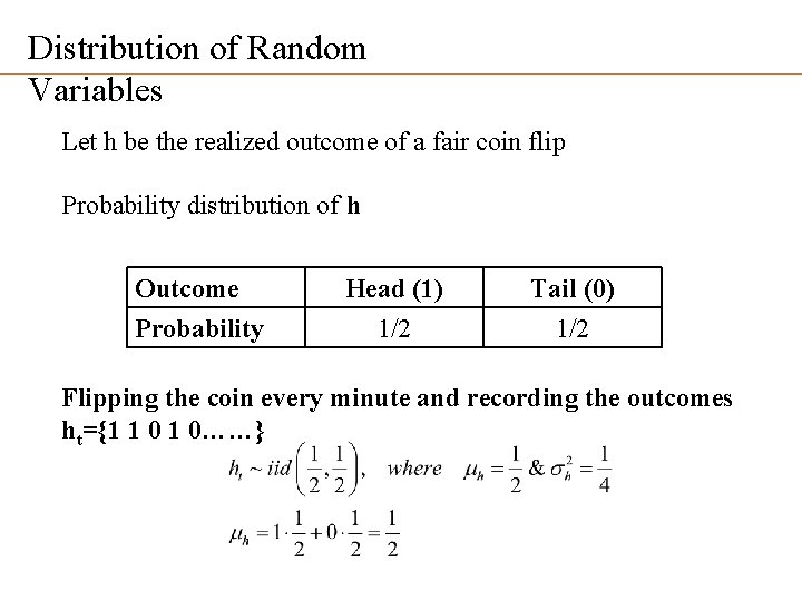
Distribution of Random Variables Let h be the realized outcome of a fair coin flip Probability distribution of h Outcome Probability Head (1) 1/2 Tail (0) 1/2 Flipping the coin every minute and recording the outcomes ht={1 1 0……}

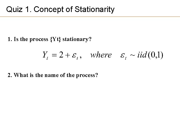
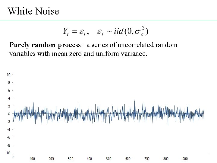
Quiz 1. Concept of Stationarity 1. Is the process {Yt} stationary? 2. What is the name of the process?

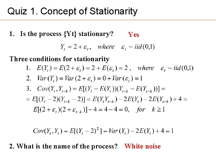
Quiz 1. Concept of Stationarity 1. Is the process {Yt} stationary? Yes Three conditions for stationarity 2. What is the name of the process? White noise

White Noise Purely random process: a series of uncorrelated random variables with mean zero and uniform variance.

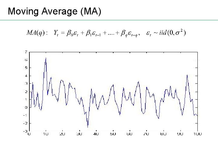
Moving Average (MA)

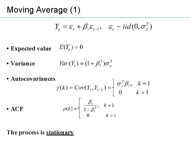
Moving Average (1) • Expected value • Variance • Autocovariances • ACF The process is stationary

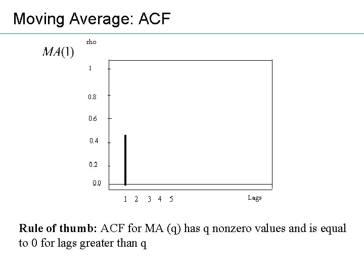
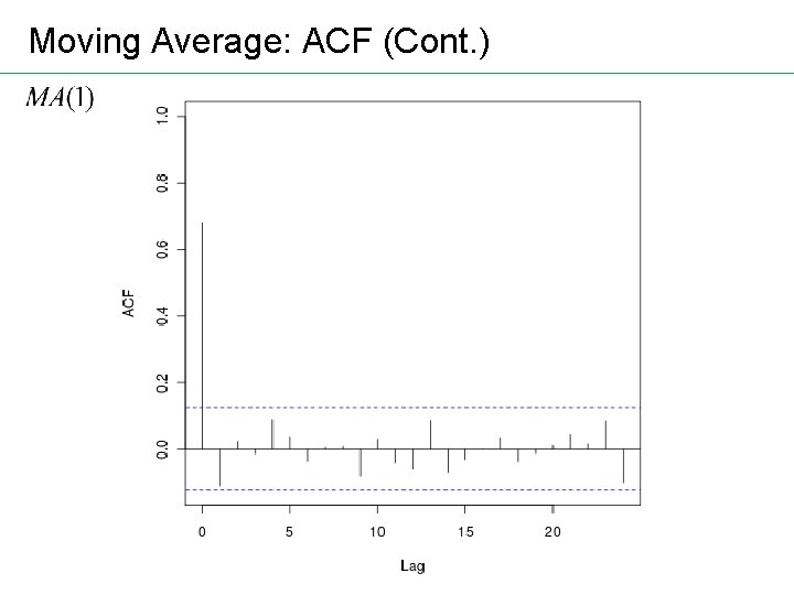
Moving Average: ACF Rule of thumb: ACF for MA (q) has q nonzero values and is equal to 0 for lags greater than q

Moving Average: ACF (Cont. )

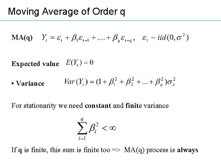
Moving Average of Order q MA(q) Expected value • Variance For stationarity we need constant and finite variance If q is finite, this sum is finite too => MA(q) process is always

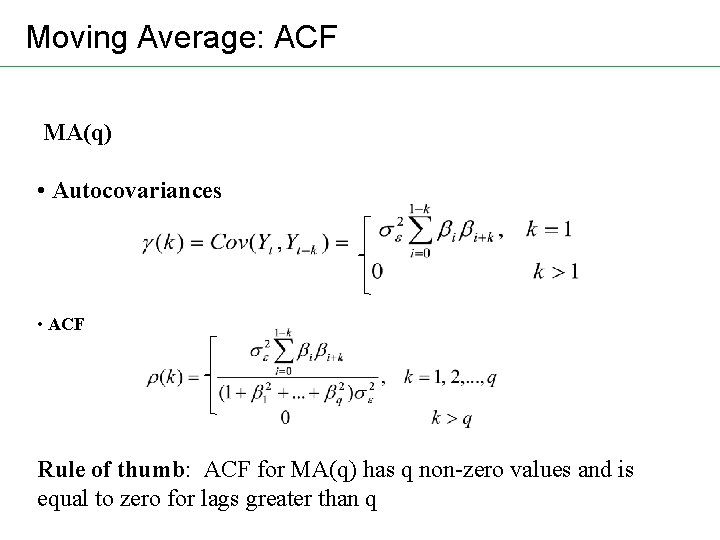
Moving Average: ACF MA(q) • Autocovariances • ACF Rule of thumb: ACF for MA(q) has q non-zero values and is equal to zero for lags greater than q

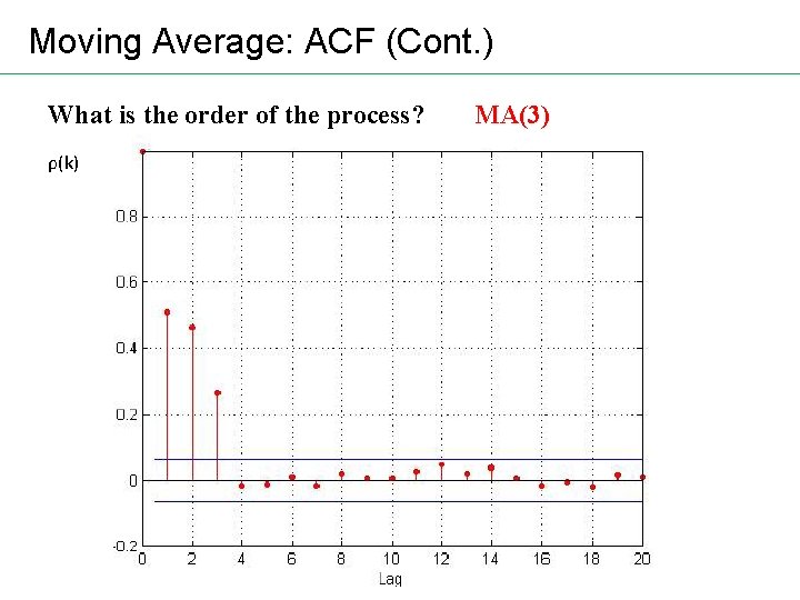
Moving Average: ACF (Cont. ) What is the order of the process? ρ(k) MA(3)

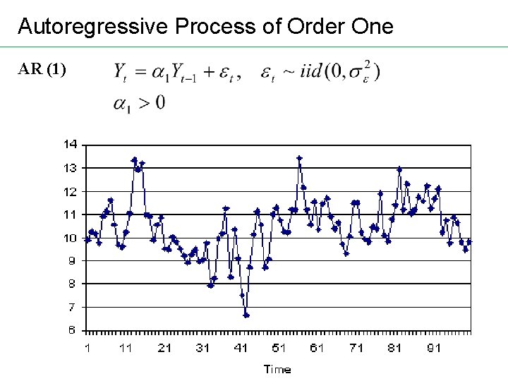
Autoregressive Process of Order One AR (1)

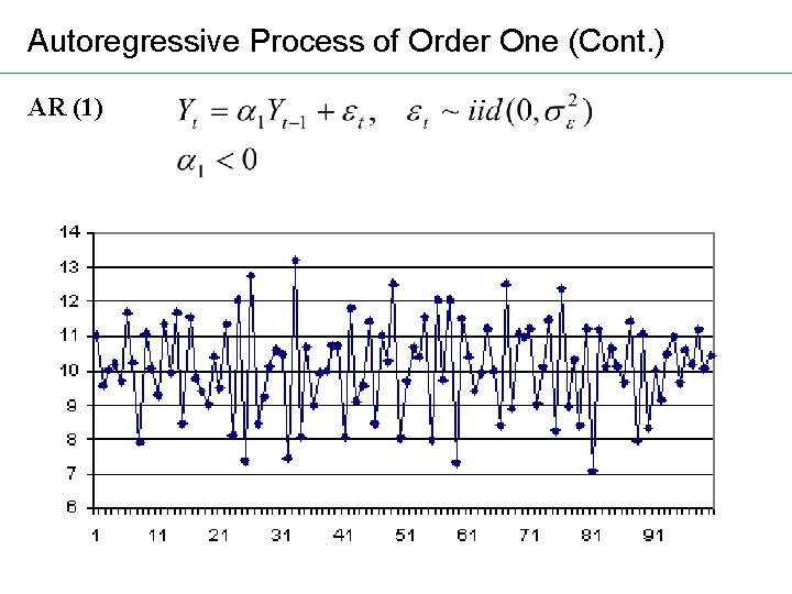
Autoregressive Process of Order One (Cont. ) AR (1)

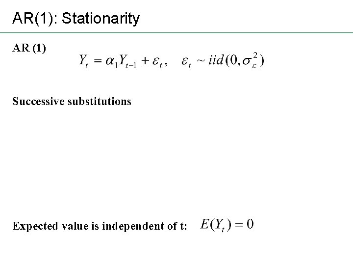
AR(1): Stationarity AR (1) Successive substitutions Expected value is independent of t:

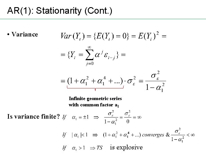
AR(1): Stationarity (Cont. ) • Variance Infinite geometric series with common factor a 1 Is variance finite? is explosive

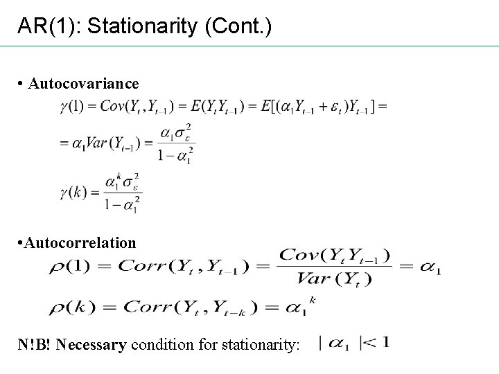
AR(1): Stationarity (Cont. ) • Autocovariance • Autocorrelation N!B! Necessary condition for stationarity:

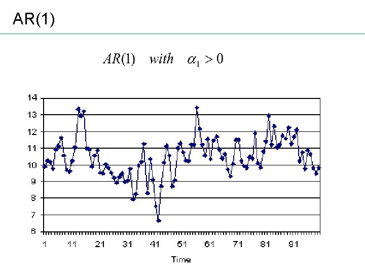
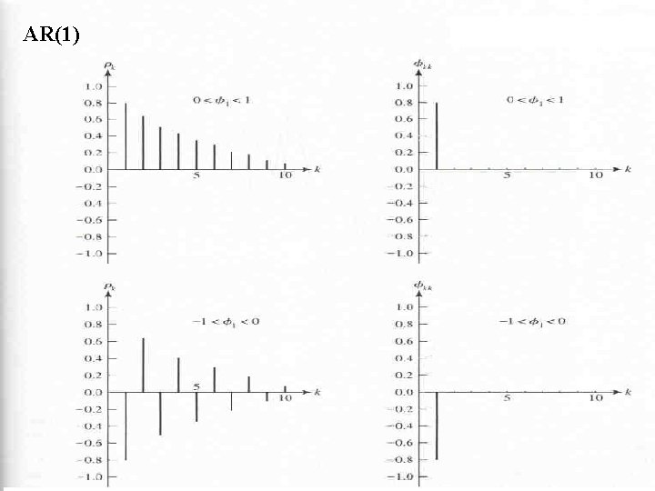
AR(1)

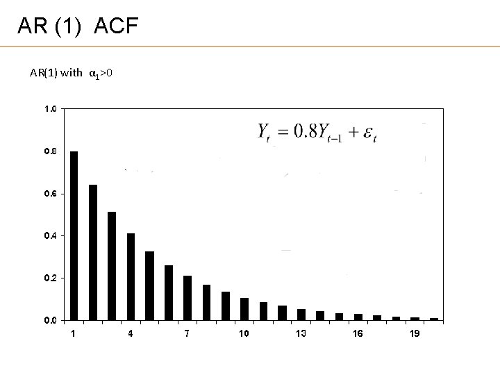
AR (1) ACF AR(1) with α 1>0

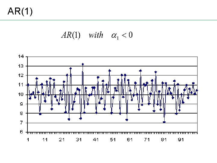
AR(1)

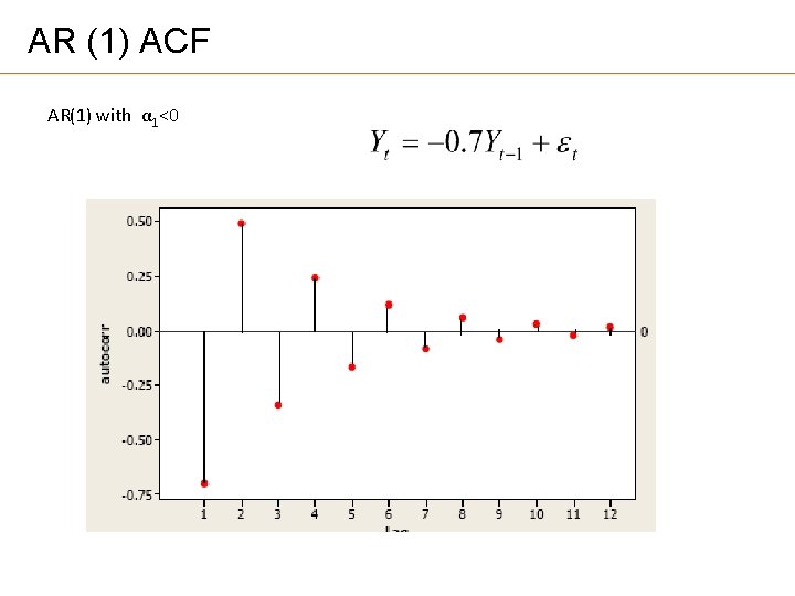
AR (1) ACF AR(1) with α 1<0

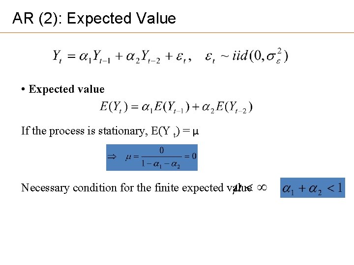
AR (2): Expected Value • Expected value If the process is stationary, E(Y t) = μ Necessary condition for the finite expected value is

AR (2): Variance is timeinvariant

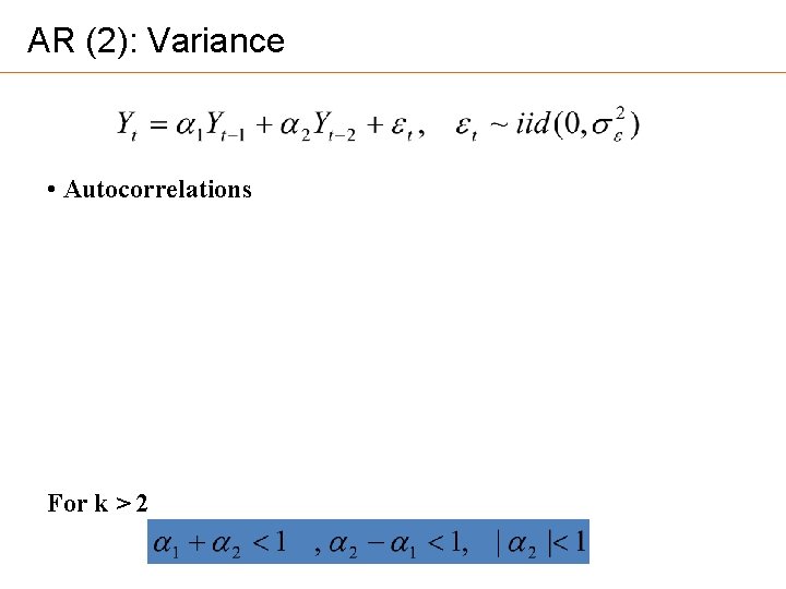
AR (2): Variance • Autocorrelations For k > 2

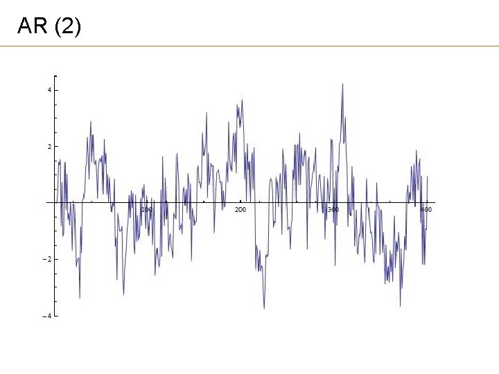
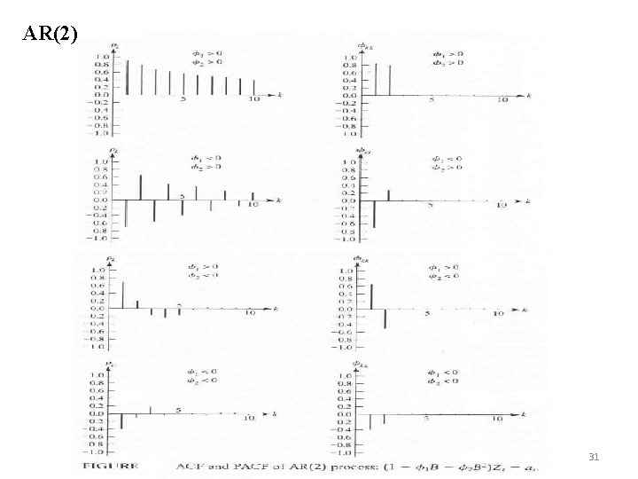
AR (2)

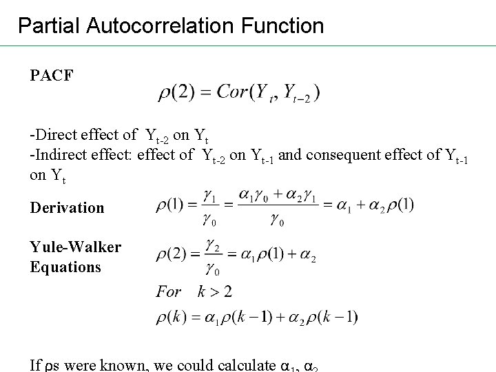
Partial Autocorrelation Function PACF -Direct effect of Yt-2 on Yt -Indirect effect: effect of Yt-2 on Yt-1 and consequent effect of Yt-1 on Yt Derivation Yule-Walker Equations If ρs were known, we could calculate α , α

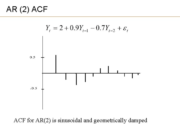
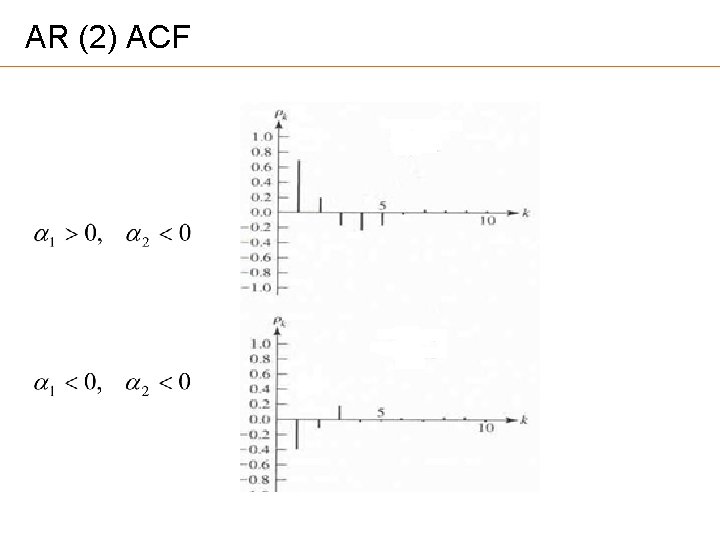
AR (2) ACF for AR(2) is sinusoidal and geometrically damped

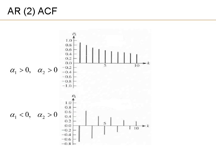
AR (2) ACF

AR (2) ACF

AR(1) 30

AR(2) 31

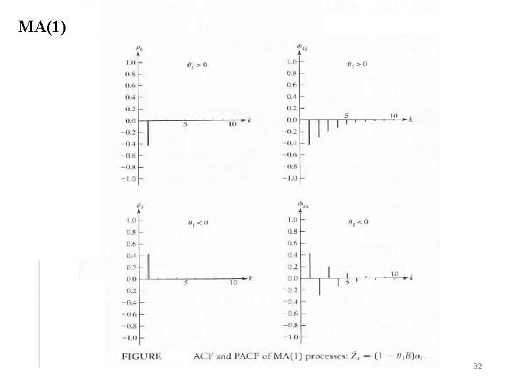
MA(1) 32

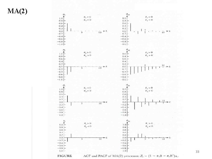
MA(2) 33

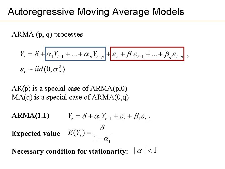
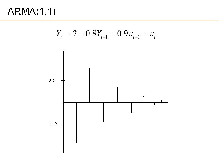
Autoregressive Moving Average Models ARMA (p, q) processes AR(p) is a special case of ARMA(p, 0) MA(q) is a special case of ARMA(0, q) ARMA(1, 1) Expected value Necessary condition for stationarity:

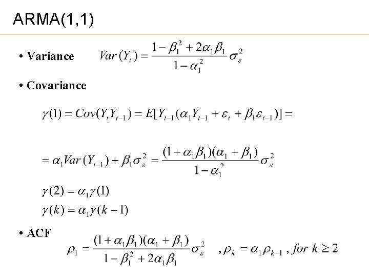
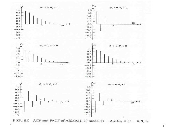
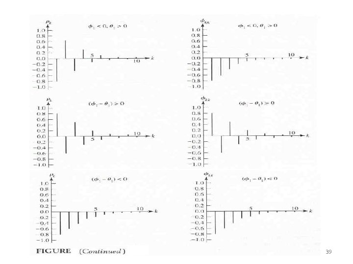
ARMA(1, 1) • Variance • Covariance • ACF

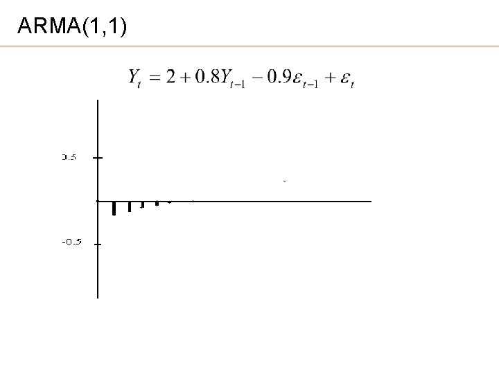
ARMA(1, 1)

ARMA(1, 1)

38

39

Next Lecture Topic: Non-Stationary TS and Transformation to Stationarity ! Reading assignment for next week Enders , Chapter 2, pp. 67 -82. Deriving variance, covariances and correlations for AR (1)-(2), MA(1)-(2), and ARMA(1, 1).