Data Science and Big Data Analytics Chap 8

Data Science and Big Data Analytics Chap 8: Adv Analytical Theory and Methods: Time Series Analysis Charles Tappert Seidenberg School of CSIS, Pace University

Chapter Sections n 8. 1 Overview of Time Series Analysis n n 8. 2 ARIMA Model n n n n 8. 1. 1 Box-Jenkins Methodology 8. 2. 1 8. 2. 2 8. 2. 3 8. 2. 4 8. 2. 5 8. 2. 6 Autocorrelation Function (ACF) Autoregressive Models Moving Average Models ARMA and ARIMA Models Building and Evaluating an ARIMA Model Reasons to Choose and Cautions 8. 3 Additional Methods Summary

8 Time Series Analysis n This chapter’s emphasis is on Identifying the underlying structure of the time series n Fitting an appropriate Autoregressive Integrated Moving Average (ARIMA) model n

8. 1 Overview of Time Series Analysis n n n Time series analysis attempts to model the underlying structure of observations over time A time series, Y = a+ b. X , is an ordered sequence of equally spaced values over time The analyses presented in this chapter are limited to equally spaced time series of one variable

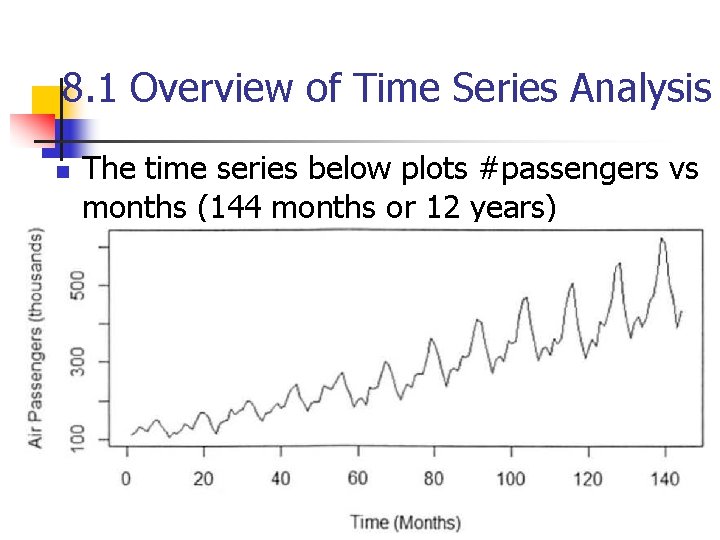
8. 1 Overview of Time Series Analysis n The time series below plots #passengers vs months (144 months or 12 years)

8. 1 Overview of Time Series Analysis n The goals of time series analysis are n n n Identify and model the structure of the time series Forecast future values in the time series Time series analysis has many applications in finance, economics, biology, engineering, retail, and manufacturing

8. 1 Overview of Time Series Analysis 8. 1. 1 Box-Jenkins Methodology n A time series can consist of the components: n Trend – long-term movement in a time series, increasing or decreasing over time – for example, n n n Seasonality – describes the fixed, periodic fluctuation in the observations over time n n Usually related to the calendar – e. g. , airline passenger example Cyclic – also periodic but not as fixed n n Steady increase in sales month over month Annual decline of fatalities due to car accidents E. g. , retail sales versus the boom-bust cycle of the economy Random – is what remains, usually noise n This structure is what is modeled to obtain forecasts

8. 1 Overview of Time Series Analysis 8. 1. 1 Box-Jenkins Methodology n The Box-Jenkins methodology has three main steps: 1. Condition the data and select a model n n Estimate the model parameters 3. Assess the model, return to Step 1 if necessary This chapter uses the Box-Jenkins methodology to apply an ARIMA model to a given time series 2. n Identify/account for trends/seasonality in time series Examine remaining time series to determine a model

8. 1 Overview of Time Series Analysis 8. 1. 1 Box-Jenkins Methodology n n Most of this chapter is rather advanced and only the basics will be tested on in this course We could skip the remainder of the chapter’s slides

8. 2 ARIMA Model ARIMA = Autoregressive Integrated Moving Average n n n Step 1: remove any trends/seasonality in time series Achieve a time series with certain properties to which autoregressive and moving average models can be applied Such a time series is known as a stationary time series

8. 2 ARIMA Model ARIMA = Autoregressive Integrated Moving Average n Time series yt for t= 1, 2, 3, . . . t is stationary if the following three conditions are met 1. 2. 3. The expected value of yt is constant for all t The variance of yt is finite The covariance of yt and yt+h depends only on the value of h = 0, 1, 2, . . . for all t n The covariance of yt and yt+h is a measure of how the two variables yt and yt+h vary together

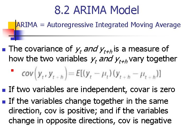
8. 2 ARIMA Model ARIMA = Autoregressive Integrated Moving Average n The covariance of yt and yt+h is a measure of how the two variables yt and yt+h vary together n n n If two variables are independent, covar is zero If the variables change together in the same direction, cov is positive; and if the variables change in opposite directions, cov is negative

8. 2 ARIMA Model ARIMA = Autoregressive Integrated Moving Average n A stationary time series, by condition (1), has constant mean, say m, so covariance simplifies to n n By condition (3), cov between two points can be nonzero, but cov is only function of h – e. g. , h=3 n n If h=0, cov(0) = cov(yt, yt) = var(yt) for all t

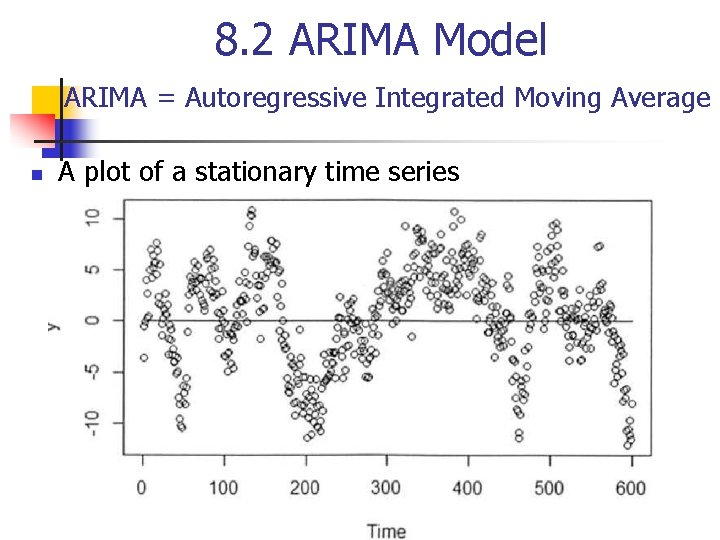
8. 2 ARIMA Model ARIMA = Autoregressive Integrated Moving Average n A plot of a stationary time series

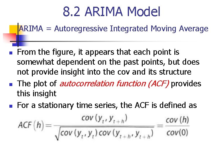
8. 2 ARIMA Model ARIMA = Autoregressive Integrated Moving Average n n n From the figure, it appears that each point is somewhat dependent on the past points, but does not provide insight into the cov and its structure The plot of autocorrelation function (ACF) provides this insight For a stationary time series, the ACF is defined as

8. 2 ARIMA Model ARIMA = Autoregressive Integrated Moving Average n n Because the cov(0) is the variance, the ACF is analogous to the correlation function of two variables, corr (yt , yt+h), and the value of the ACF falls between -1 and 1 Thus, the closer the absolute value of ACF(h) is to 1, the more useful yt can be as a predictor of yt+h

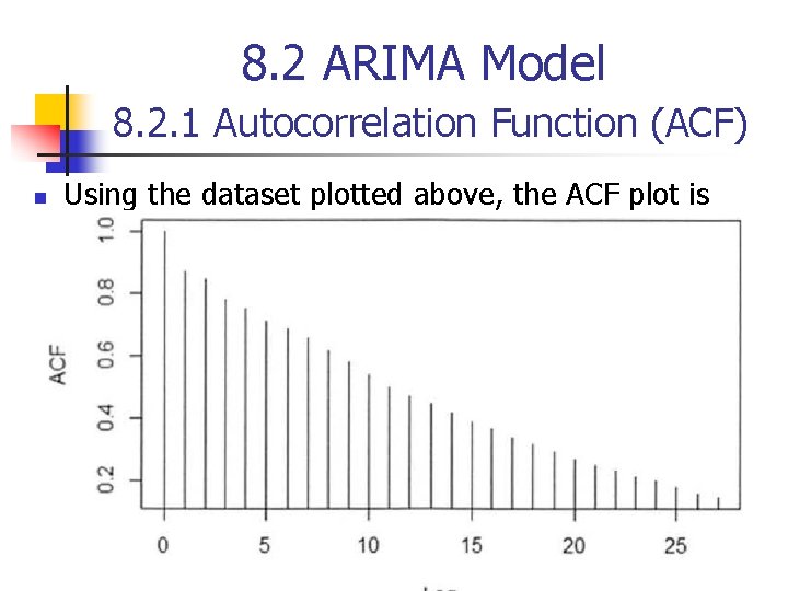
8. 2 ARIMA Model 8. 2. 1 Autocorrelation Function (ACF) n Using the dataset plotted above, the ACF plot is

8. 2 ARIMA Model 8. 2. 1 Autocorrelation Function (ACF) n By convention, the quantity h in the ACF is referred to as the lag, the difference between the time points t and t + h n n At lag 0, the ACF provides the correlation of every point with itself According to the ACF plot, at lag 1 the correlation between yt and yt-1 is approximately 0. 9, which is very close to 1, so yt-1 appears to be a good predictor of the value of yt 1 n In other words, a model can be considered that would express yt as a linear sum of its previous 8 terms. Such a model is known as an autoregressive model of order 8

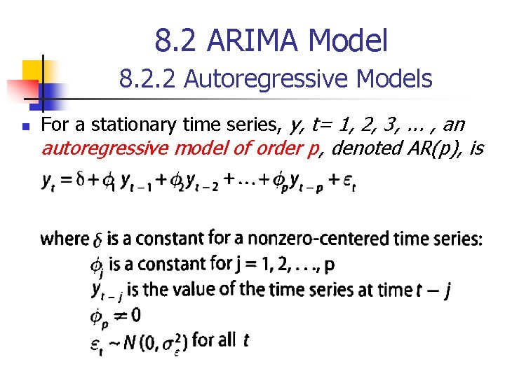
8. 2 ARIMA Model 8. 2. 2 Autoregressive Models n For a stationary time series, y, t= 1, 2, 3, . . . , an autoregressive model of order p, denoted AR(p), is

8. 2 ARIMA Model 8. 2. 2 Autoregressive Models n n Thus, a particular point in the time series can be expressed as a linear combination of the prior p values, yt-j for j = 1, 2, . . . p, of the time series plus a random error term, et The et in the time series is often called a white noise process that represents random, independent fluctuations that are part of the time series

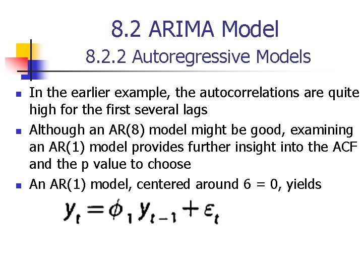
8. 2 ARIMA Model 8. 2. 2 Autoregressive Models n n n In the earlier example, the autocorrelations are quite high for the first several lags Although an AR(8) model might be good, examining an AR(1) model provides further insight into the ACF and the p value to choose An AR(1) model, centered around 6 = 0, yields

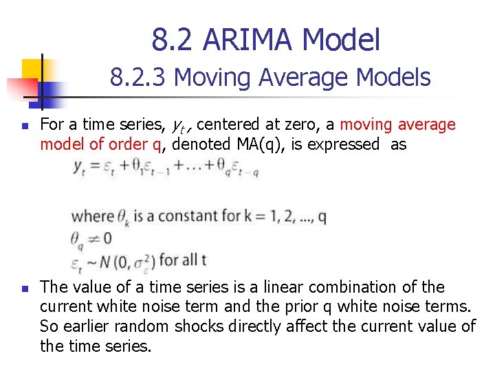
8. 2 ARIMA Model 8. 2. 3 Moving Average Models n n For a time series, yt , centered at zero, a moving average model of order q, denoted MA(q), is expressed as The value of a time series is a linear combination of the current white noise term and the prior q white noise terms. So earlier random shocks directly affect the current value of the time series.

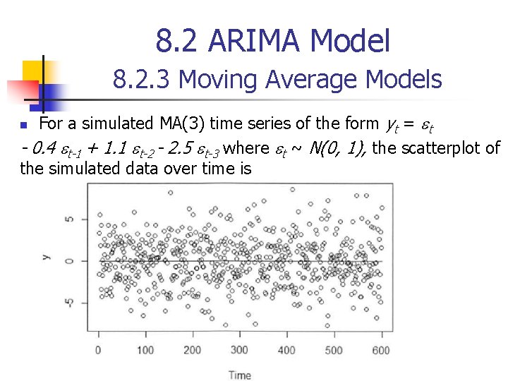
8. 2 ARIMA Model 8. 2. 3 Moving Average Models For a simulated MA(3) time series of the form yt = et - 0. 4 et-1 + 1. 1 et-2 - 2. 5 et-3 where et ~ N(0, 1), the scatterplot of the simulated data over time is n

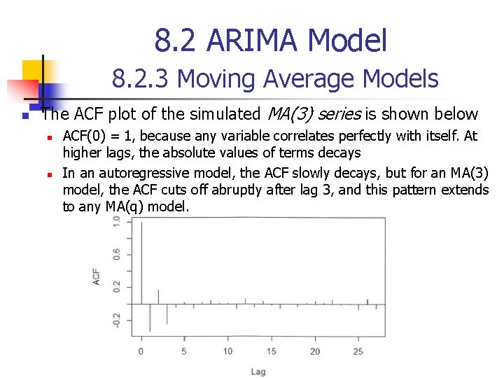
8. 2 ARIMA Model 8. 2. 3 Moving Average Models n The ACF plot of the simulated MA(3) series is shown below n n ACF(0) = 1, because any variable correlates perfectly with itself. At higher lags, the absolute values of terms decays In an autoregressive model, the ACF slowly decays, but for an MA(3) model, the ACF cuts off abruptly after lag 3, and this pattern extends to any MA(q) model.

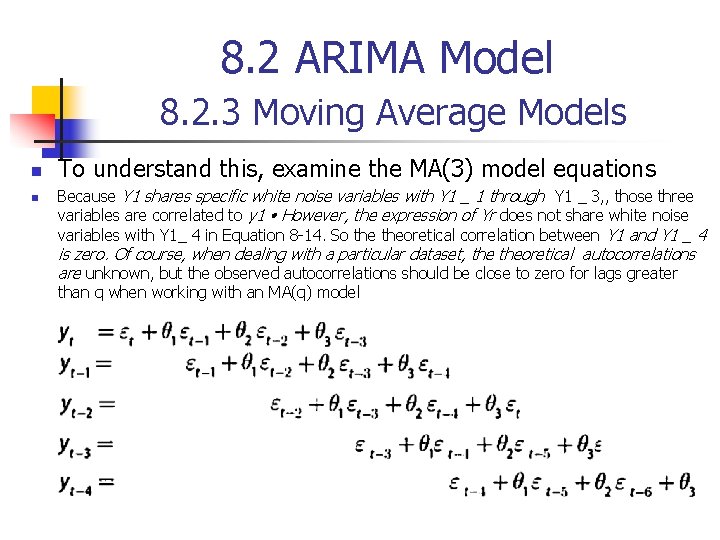
8. 2 ARIMA Model 8. 2. 3 Moving Average Models n n To understand this, examine the MA(3) model equations Because Y 1 shares specific white noise variables with Y 1 _ 1 through Y 1 _ 3, , those three variables are correlated to y 1 • However, the expression of Yr does not share white noise variables with Y 1_ 4 in Equation 8 -14. So theoretical correlation between Y 1 and Y 1 _ 4 is zero. Of course, when dealing with a particular dataset, theoretical autocorrelations are unknown, but the observed autocorrelations should be close to zero for lags greater than q when working with an MA(q) model

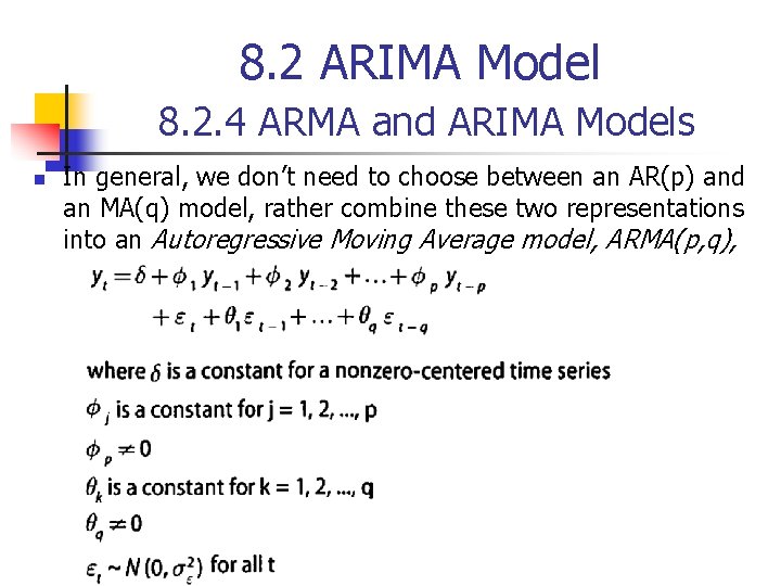
8. 2 ARIMA Model 8. 2. 4 ARMA and ARIMA Models n In general, we don’t need to choose between an AR(p) and an MA(q) model, rather combine these two representations into an Autoregressive Moving Average model, ARMA(p, q),

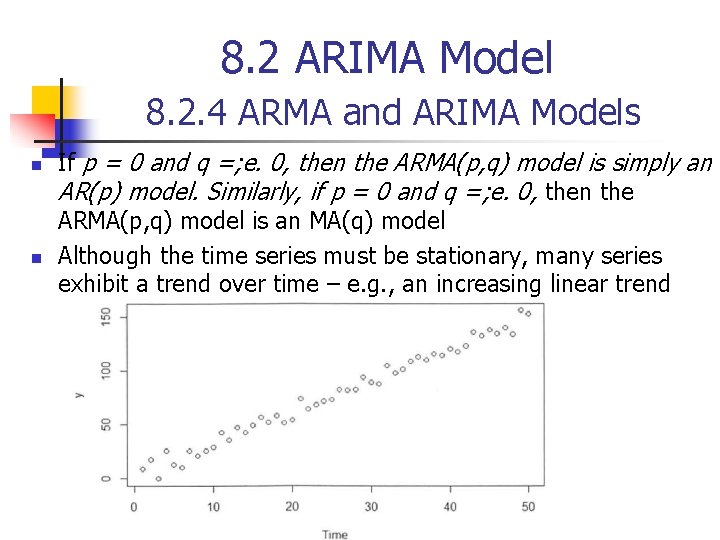
8. 2 ARIMA Model 8. 2. 4 ARMA and ARIMA Models n n If p = 0 and q =; e. 0, then the ARMA(p, q) model is simply an AR(p) model. Similarly, if p = 0 and q =; e. 0, then the ARMA(p, q) model is an MA(q) model Although the time series must be stationary, many series exhibit a trend over time – e. g. , an increasing linear trend

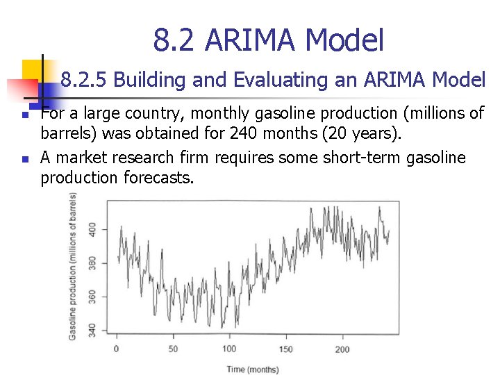
8. 2 ARIMA Model 8. 2. 5 Building and Evaluating an ARIMA Model n n For a large country, monthly gasoline production (millions of barrels) was obtained for 240 months (20 years). A market research firm requires some short-term gasoline production forecasts.

8. 2 ARIMA Model 8. 2. 5 Building and Evaluating an ARIMA Model n Comparing Fitted Time Series Models n n The arima () function in R uses Maximum Likelihood Estimation (MLE) to estimate the model coefficients. In the R output for an ARIMA model, the log-likelihood (log. L) value is provided. The values of the model coefficients are determined such that the value of the log likelihood function is maximized. Based on the log L value, the R output provides several measures that are useful for comparing the appropriateness of one fitted model against another fitted model. These measures follow: AIC (Akaike Information Criterion) AICc (Akaike Information Criterion, corrected) BIC (Bayesian Information Criterion)

8. 2 ARIMA Model 8. 2. 6 Reasons to Choose and Cautions n One advantage of ARIMA modeling is that the analysis can be based simply on historical time series data for the variable of interest. As observed in the chapter about regression (Chapter 6), various input variables need to be considered and evaluated for inclusion in the regression model for the outcome variable.

8. 3 Additional Methods n n n n n Autoregressive Moving Average with Exogenous inputs (ARM AX) is used to analyze a time series that is dependent on another time series. For example, retail demand for products can be modeled based on the previous demand combined with a weather-related time series such as temperature or rainfall. • Spectral analysis is commonly used for signal processing and other engineering applications. Speech recognition software uses such techniques to separate the signal for the spoken words from the overall signal that may include some noi se. • Generalized Autoregressive Conditionally Heteroscedastic (GARCH) is a useful model for addressing time series with nonconstant variance or volatility. GARCH is used for modeling stock market activity and price fluctuations. • Kalman filtering is useful for analyzing real-time inputs about a system that can exist in certa in states. Typica lly, there is an underlying model of how the various components of the system interact and affect each other. A Kalman filter processes the various inputs, attempts to identify the errors in the input, and predicts the cu rrent state. For example, a Kalman filter in a vehicle navigation system can process various inputs, such as speed and direction, and update the estimate of the current location. • Multivariate time series analysis examines multiple time series and their effect on each other. Vector ARIMA (VARIMA) extends ARIMA by considering a vector of several time series at a particular time, t. VARIMA can be used in marketing analyses that examine the time series related to a company's price and sa les volume as well as related time series for the competitors.

Summary n n Time series analysis is different from other statistical techniques as most statistical analyses assume the observations are independent of each other. Time series analysis addresses the case where observations are somewhat dependent on prior observations. Using differencing, ARIMA models allow nonstationary series to be transformed into stationary series to which seasonal and nonseasonal ARMA models can be applied. Once an appropriate model has been determined, future values in the time series can be forecasted.