Linear Stationary Processes ARMA models This lecture introduces

Linear Stationary Processes. ARMA models

• This lecture introduces the basic linear models for stationary processes. • Considering only stationary processes is very restrictive since most economic variables are non-stationary. • However, stationary linear models are used as building blocks in more complicated nonlinear and/or non-stationary models.

Roadmap 1. The Wold decomposition 2. From the Wold decomposition to the ARMA representation. 3. MA processes and invertibility 4. AR processes, stationarity and causality 5. ARMA, invertibility and causality.

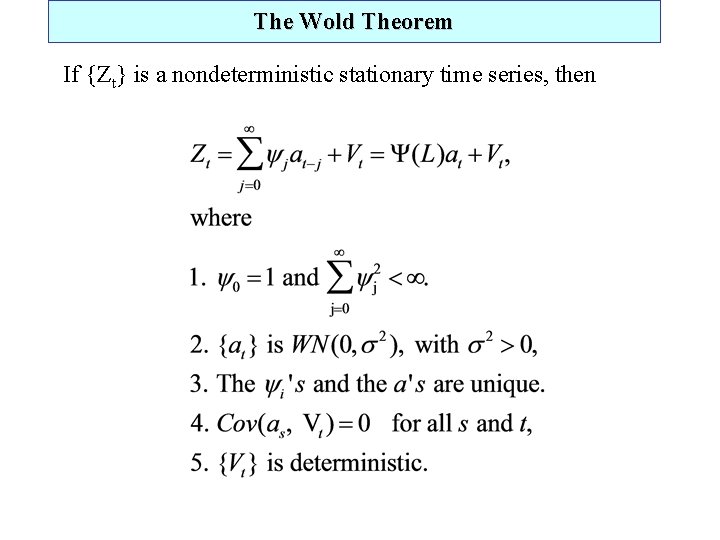
The Wold Decomposition Wold theorem in words: Any stationary process {Zt} can be expressed as a sum of two components: - a stochastic component: a linear combination of lags of a white noise process. - a deterministic component, uncorrelated with the latter stochastic component. �

The Wold Theorem If {Zt} is a nondeterministic stationary time series, then

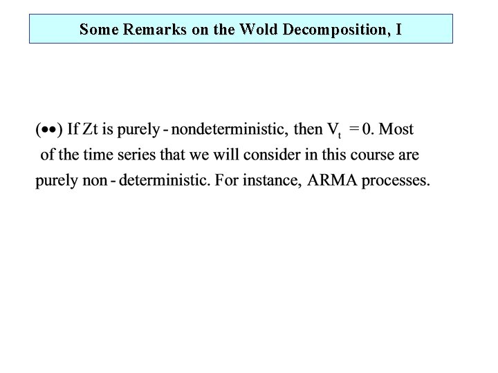
Some Remarks on the Wold Decomposition, I

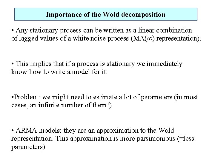
Importance of the Wold decomposition • Any stationary process can be written as a linear combination of lagged values of a white noise process (MA(∞) representation). • This implies that if a process is stationary we immediately know how to write a model for it. • Problem: we might need to estimate a lot of parameters (in most cases, an infinite number of them!) • ARMA models: they are an approximation to the Wold representation. This approximation is more parsimonious (=less parameters)

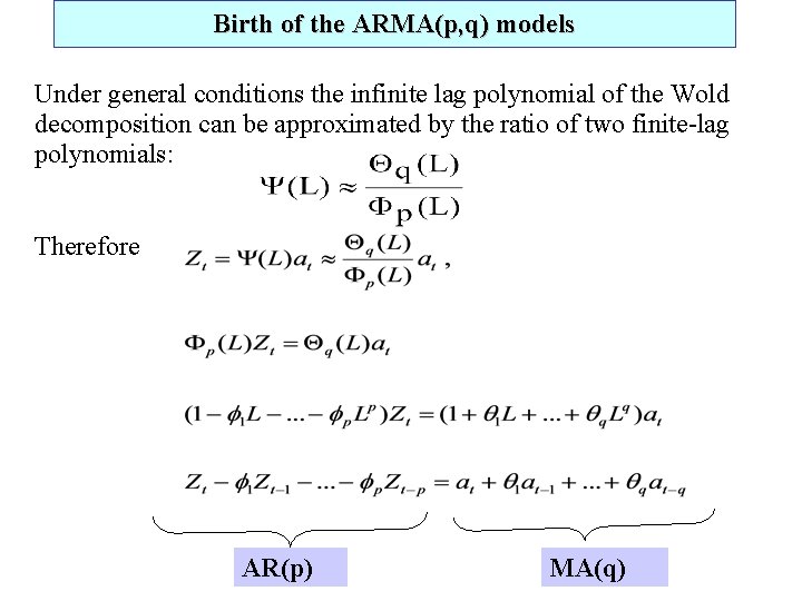
Birth of the ARMA(p, q) models Under general conditions the infinite lag polynomial of the Wold decomposition can be approximated by the ratio of two finite-lag polynomials: Therefore AR(p) MA(q)

MA processes

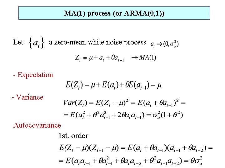
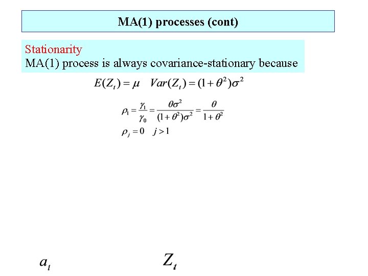
MA(1) process (or ARMA(0, 1)) Let a zero-mean white noise process - Expectation - Variance Autocovariance

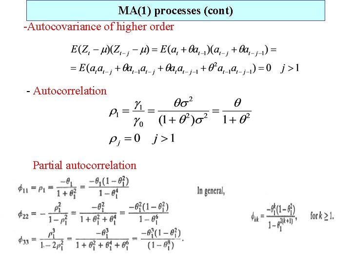
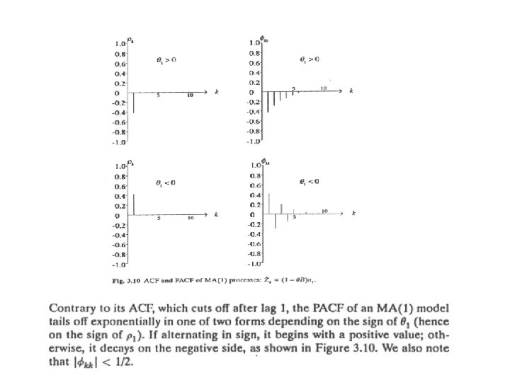
MA(1) processes (cont) -Autocovariance of higher order - Autocorrelation Partial autocorrelation

MA(1) processes (cont) Stationarity MA(1) process is always covariance-stationary because

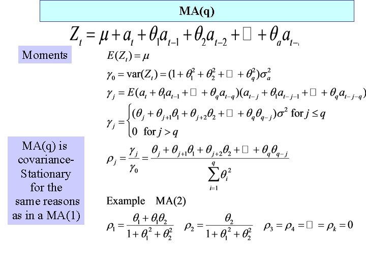
MA(q) Moments MA(q) is covariance. Stationary for the same reasons as in a MA(1)

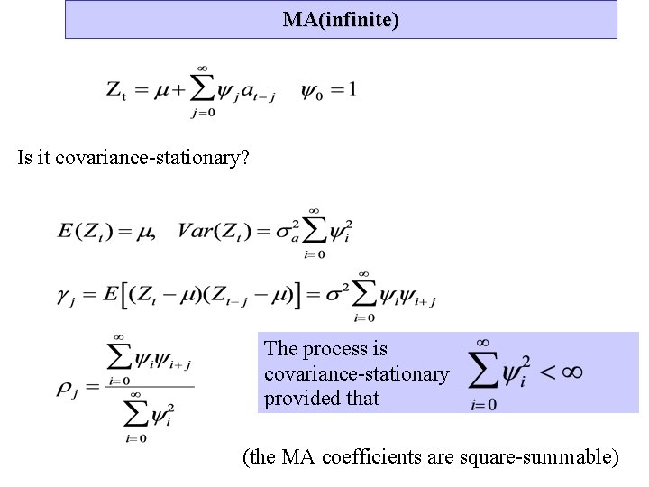
MA(infinite) Is it covariance-stationary? The process is covariance-stationary provided that (the MA coefficients are square-summable)

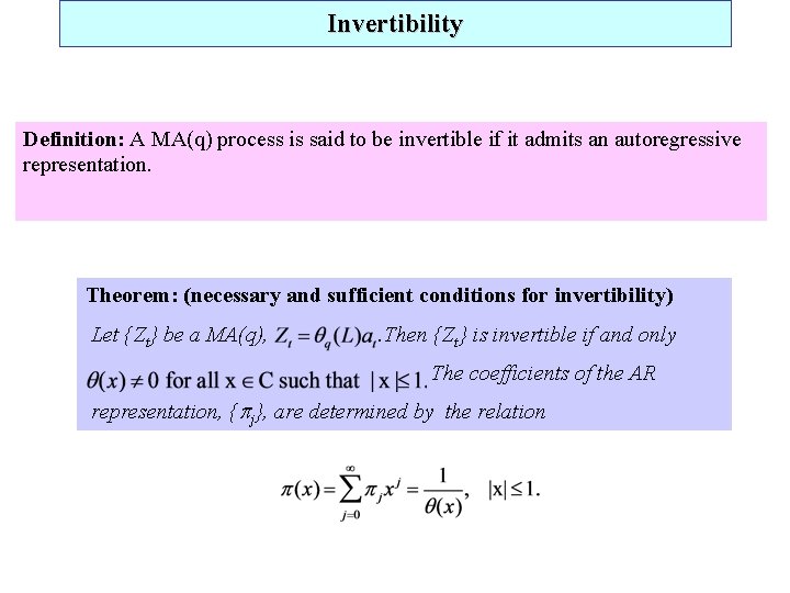
Invertibility Definition: A MA(q) process is said to be invertible if it admits an autoregressive representation. Theorem: (necessary and sufficient conditions for invertibility) Let {Zt} be a MA(q), . Then {Zt} is invertible if and only The coefficients of the AR representation, { j}, are determined by the relation

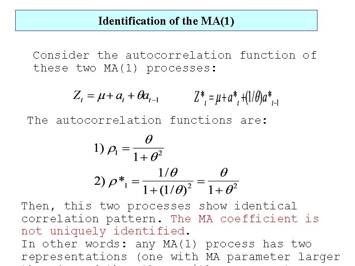
Identification of the MA(1) Consider the autocorrelation function of these two MA(1) processes: The autocorrelation functions are: Then, this two processes show identical correlation pattern. The MA coefficient is not uniquely identified. In other words: any MA(1) process has two representations (one with MA parameter larger

Identification of the MA(1) • If we identify the MA(1) through the autocorrelation structure, we would need to decide which value of to choose, the one greater than one or the one smaller than one. We prefer representations that are invertible so we will choose the value .

AR processes

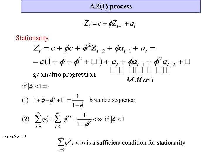
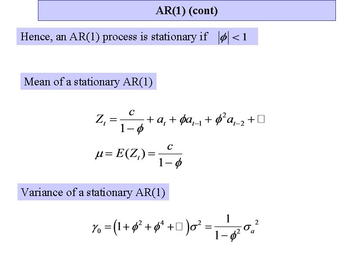
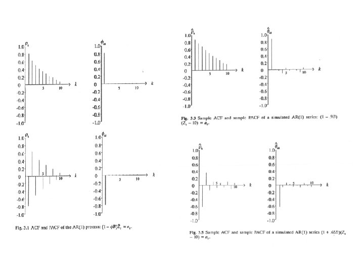
AR(1) process Stationarity geometric progression Remember!!

AR(1) (cont) Hence, an AR(1) process is stationary if Mean of a stationary AR(1) Variance of a stationary AR(1)

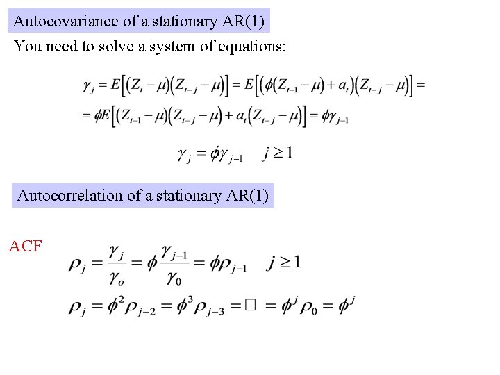
Autocovariance of a stationary AR(1) You need to solve a system of equations: Autocorrelation of a stationary AR(1) ACF

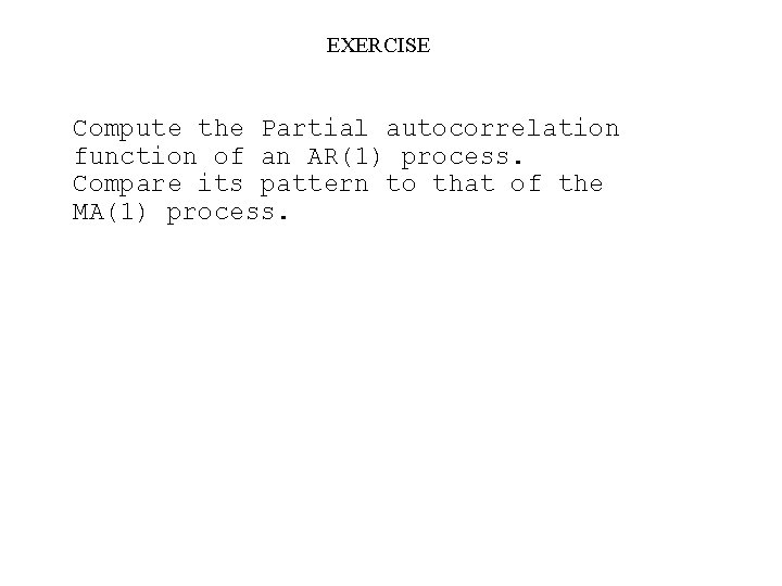
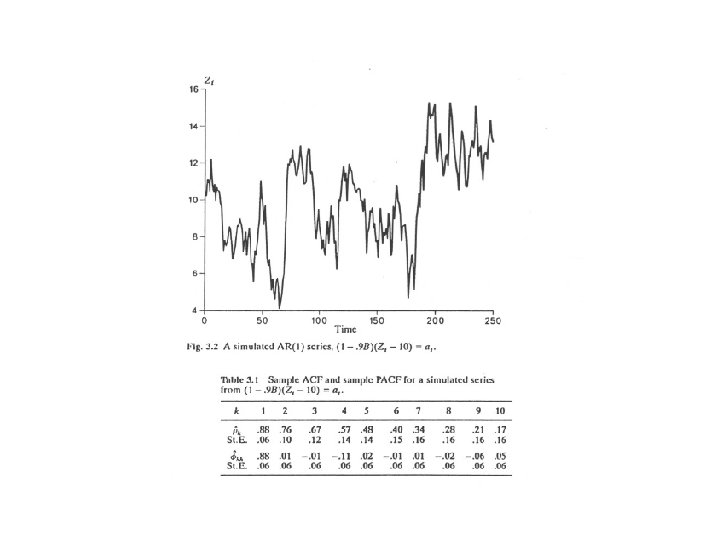
EXERCISE Compute the Partial autocorrelation function of an AR(1) process. Compare its pattern to that of the MA(1) process.

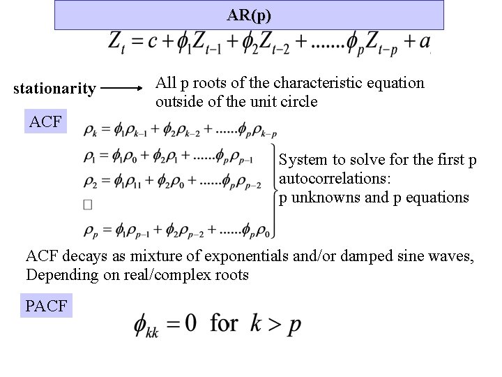
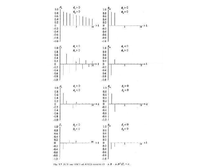
AR(p) stationarity All p roots of the characteristic equation outside of the unit circle ACF System to solve for the first p autocorrelations: p unknowns and p equations ACF decays as mixture of exponentials and/or damped sine waves, Depending on real/complex roots PACF

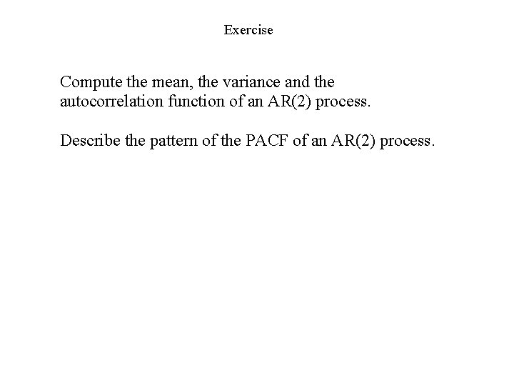
Exercise Compute the mean, the variance and the autocorrelation function of an AR(2) process. Describe the pattern of the PACF of an AR(2) process.

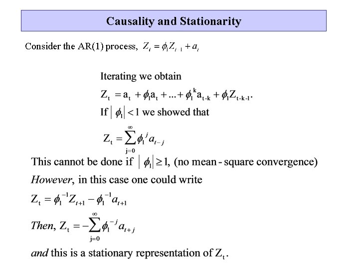
Causality and Stationarity Consider the AR(1) process,

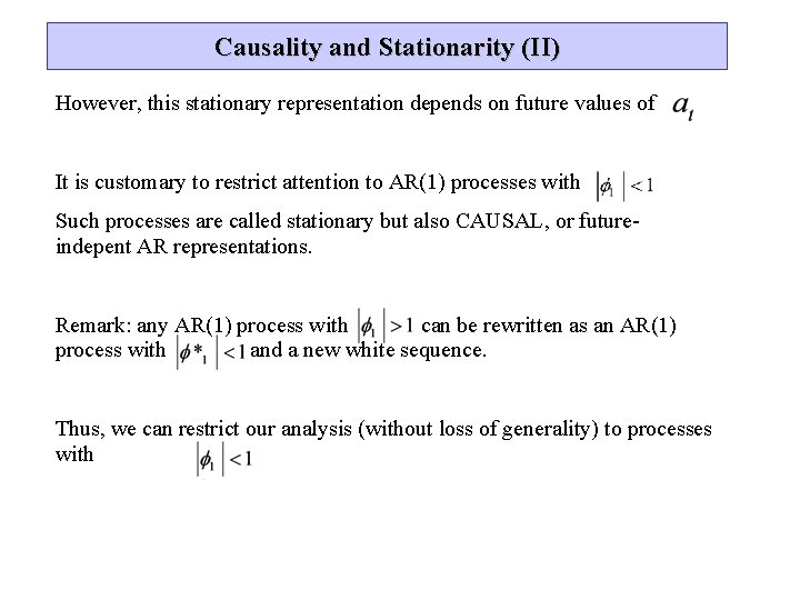
Causality and Stationarity (II) However, this stationary representation depends on future values of It is customary to restrict attention to AR(1) processes with Such processes are called stationary but also CAUSAL, or futureindepent AR representations. Remark: any AR(1) process with can be rewritten as an AR(1) process with and a new white sequence. Thus, we can restrict our analysis (without loss of generality) to processes with

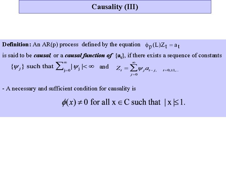
Causality (III) Definition: An AR(p) process defined by the equation is said to be causal, or a causal function of {at}, if there exists a sequence of constants and - A necessary and sufficient condition for causality is

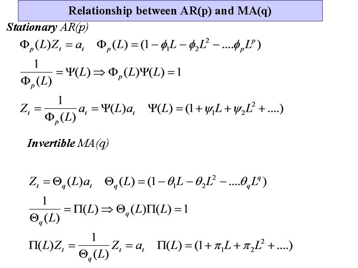
Relationship between AR(p) and MA(q) Stationary AR(p) Invertible MA(q)

ARMA(p, q) Processes

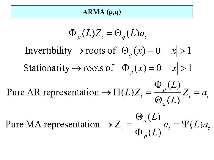
ARMA (p, q)

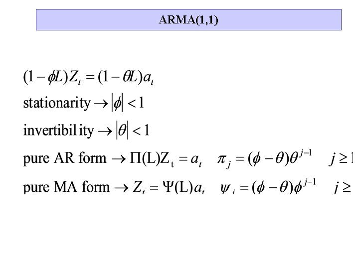
ARMA(1, 1)

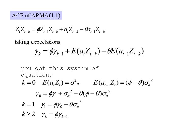
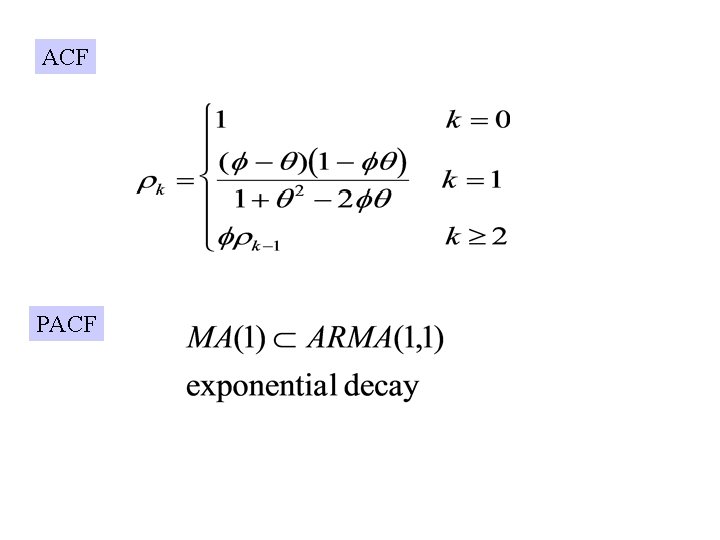
ACF of ARMA(1, 1) taking expectations you get this system of equations

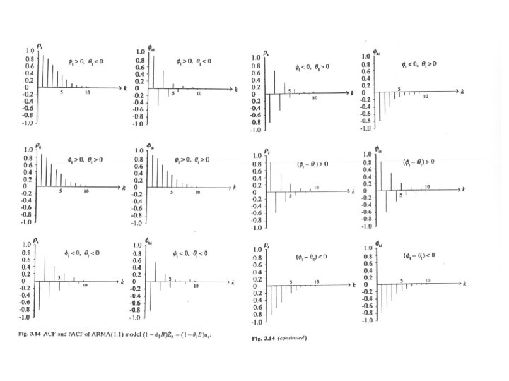
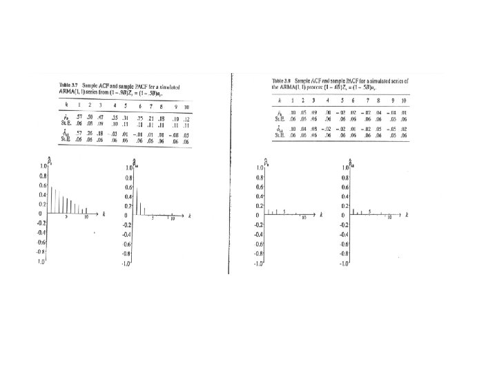
ACF PACF

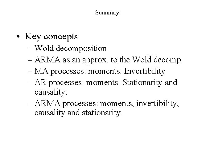
Summary • Key concepts – Wold decomposition – ARMA as an approx. to the Wold decomp. – MA processes: moments. Invertibility – AR processes: moments. Stationarity and causality. – ARMA processes: moments, invertibility, causality and stationarity.