
Chapter 3 ARMA Time Series Models NOTE Some





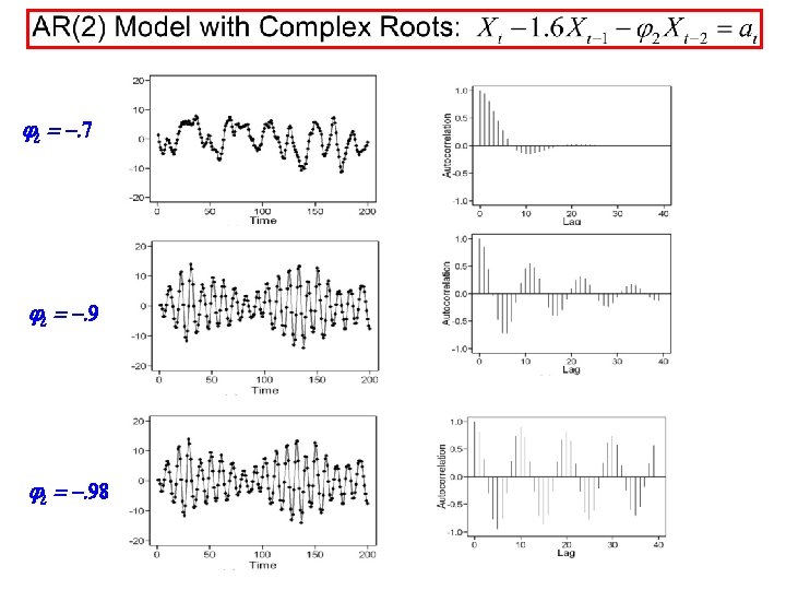
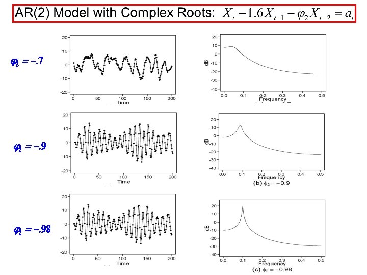





- Slides: 144
Chapter 3 ARMA Time Series Models NOTE: Some slides have blank sections. They are based on a teaching style in which the corresponding blank (derivations, theorem proofs, examples, …) are worked out in class on the board or overhead projector.
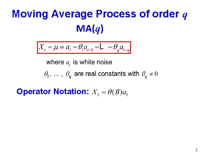
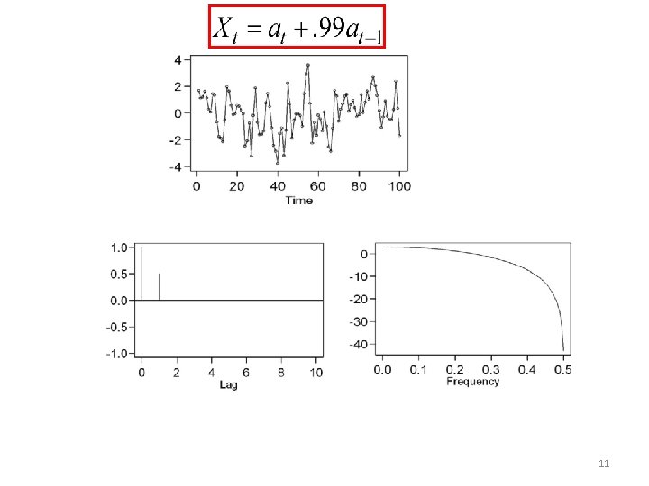
Moving Average Process of order q MA(q) Operator Notation: 2
Note: An MA(q) is a GLP with a finite number of terms 3
Stationarity Region: - range of parameters for which the resulting model is stationary Stationarity Region for an MA(q): 4
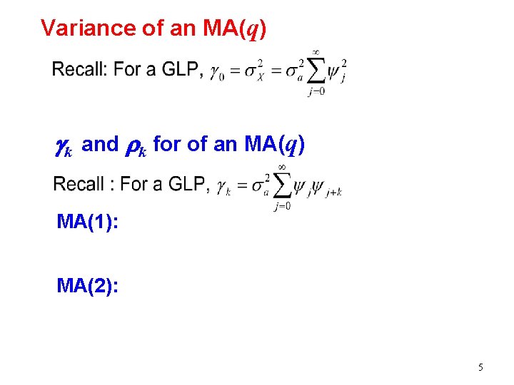
Variance of an MA(q) gk and rk for of an MA(q) MA(1): MA(2): 5
6
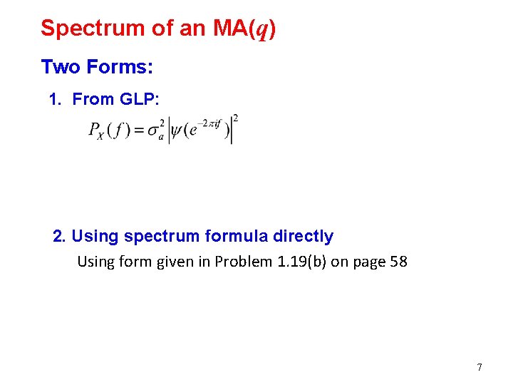
Spectrum of an MA(q) Two Forms: 1. From GLP: 2. Using spectrum formula directly Using form given in Problem 1. 19(b) on page 58 7
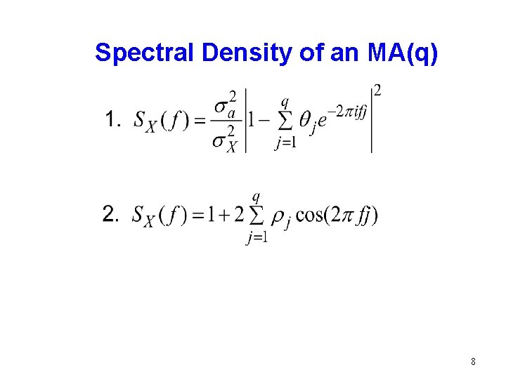
Spectral Density of an MA(q) 8
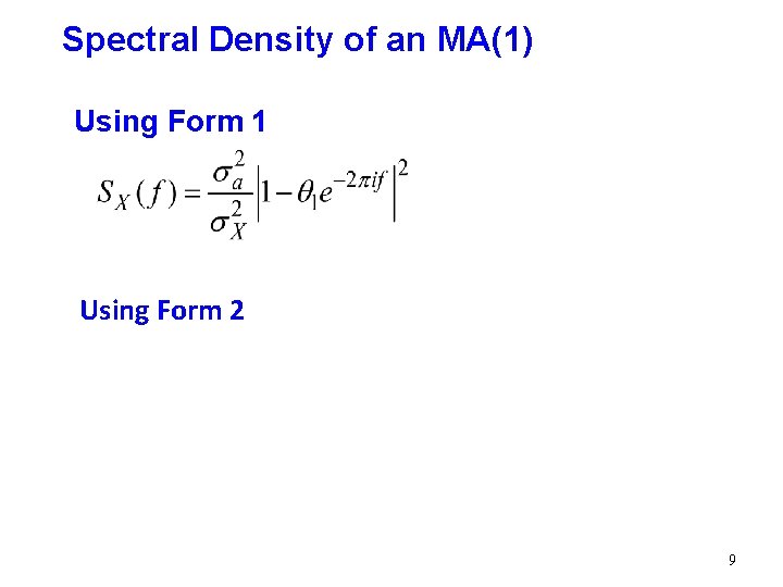
Spectral Density of an MA(1) Using Form 1 Using Form 2 9
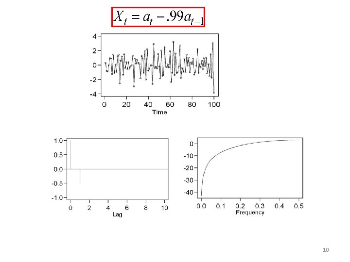
10
11
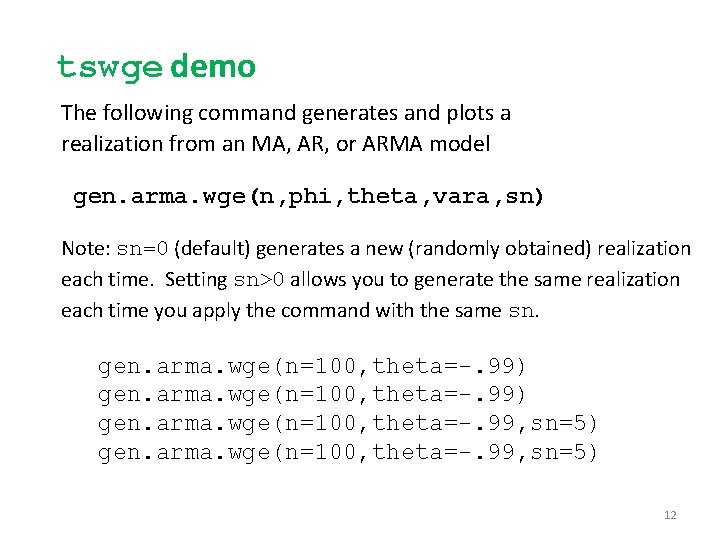
tswge demo The following command generates and plots a realization from an MA, AR, or ARMA model gen. arma. wge(n, phi, theta, vara, sn) Note: sn=0 (default) generates a new (randomly obtained) realization each time. Setting sn>0 allows you to generate the same realization each time you apply the command with the same sn. gen. arma. wge(n=100, theta=-. 99) gen. arma. wge(n=100, theta=-. 99, sn=5) 12
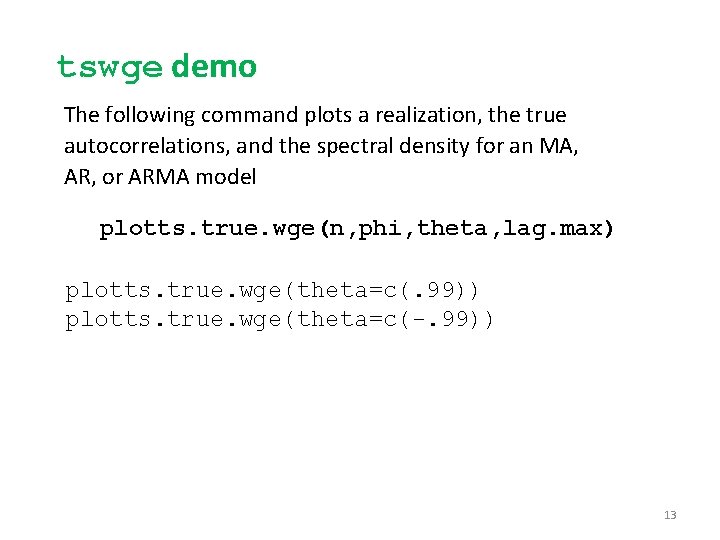
tswge demo The following command plots a realization, the true autocorrelations, and the spectral density for an MA, AR, or ARMA model plotts. true. wge(n, phi, theta, lag. max) plotts. true. wge(theta=c(. 99)) plotts. true. wge(theta=c(-. 99)) 13
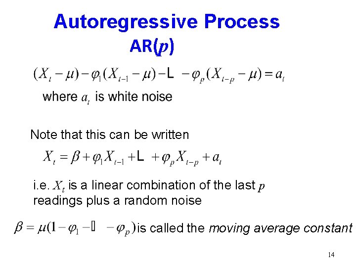
Autoregressive Process AR(p) Note that this can be written i. e. X t is a linear combination of the last p readings plus a random noise is called the moving average constant 14
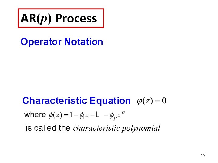
AR(p) Process Operator Notation Characteristic Equation is called the characteristic polynomial 15
Definition 3. 2 Suppose Xt is a causal, stationary process satisfying j(B)(Xt -m) = at. Then Xt will be called an AR(p) process - we will often use the zero mean form for notational simplicity
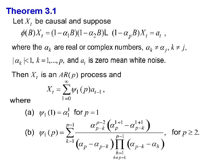
Theorem 3. 1
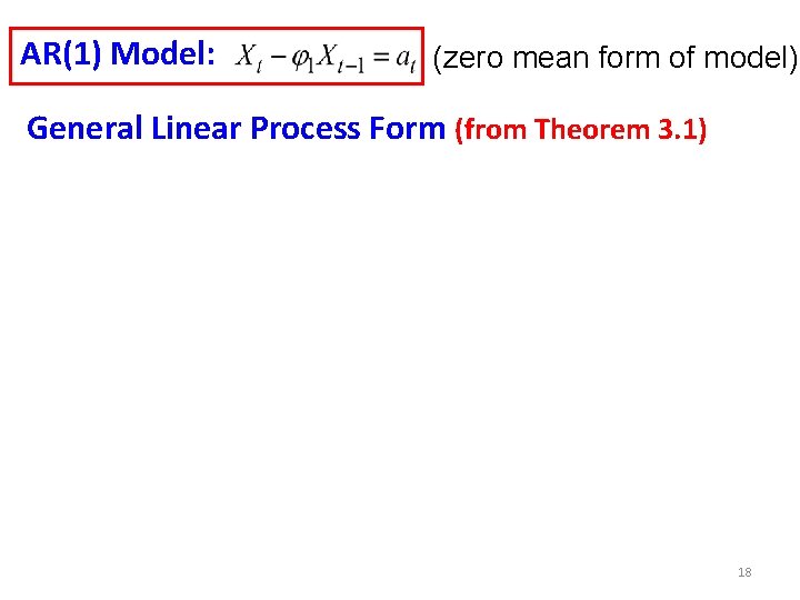
AR(1) Model: (zero mean form of model) General Linear Process Form (from Theorem 3. 1) 18
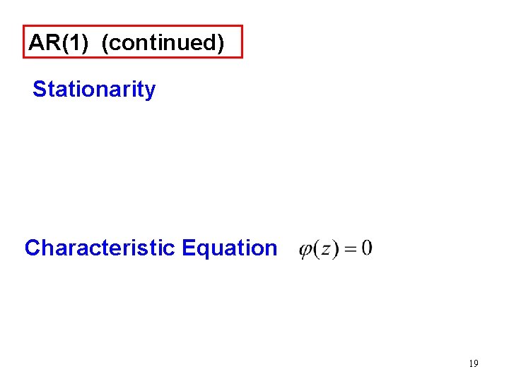
AR(1) (continued) Stationarity Characteristic Equation 19
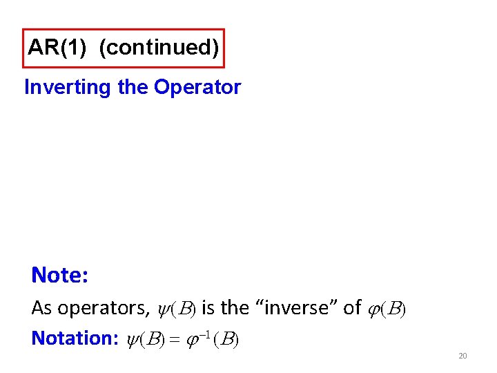
AR(1) (continued) Inverting the Operator Note: As operators, y (B) is the “inverse” of j (B) Notation: y (B) = j -1 (B) 20
In general: i. e. an AR(p) is an “infinite order MA” Note: The inverse operator is defined analogously to the inverse algebraic counterpart. General result proved in Brockwell and Davis (Time Series: Theory and Methods, 1991 - yellow book) 21
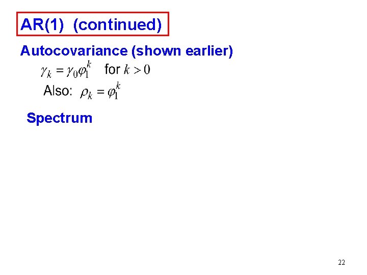
AR(1) (continued) Autocovariance (shown earlier) Spectrum 22
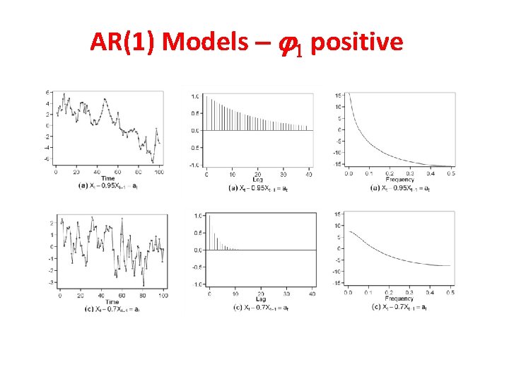
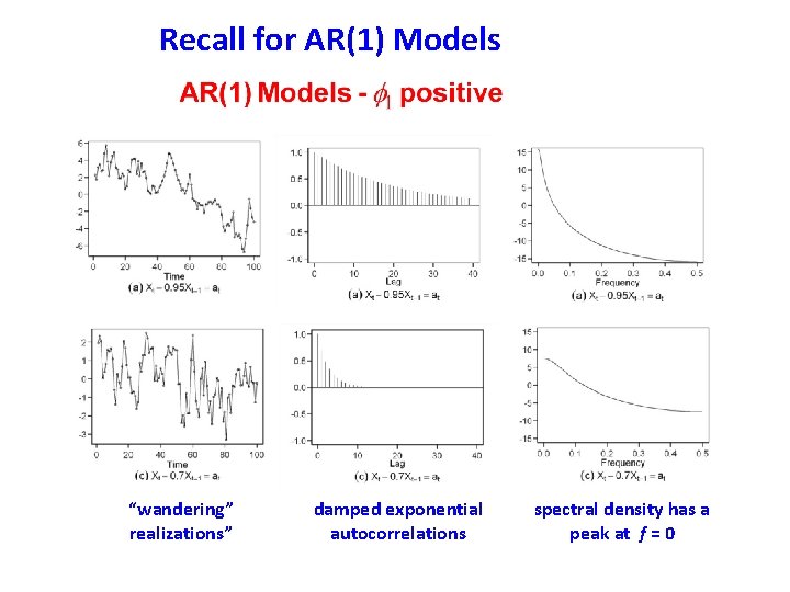
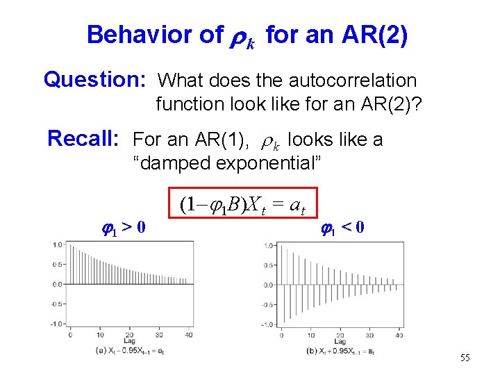
AR(1) Models j 1 positive
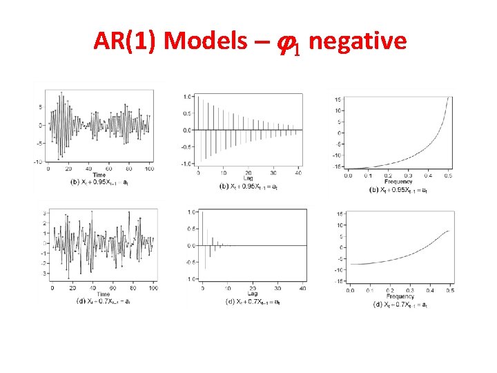
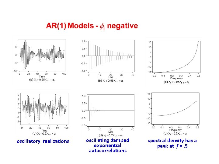
AR(1) Models j 1 negative
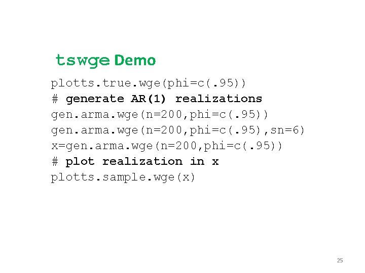
tswge Demo plotts. true. wge(phi=c(. 95)) # generate AR(1) realizations gen. arma. wge(n=200, phi=c(. 95)) gen. arma. wge(n=200, phi=c(. 95), sn=6) x=gen. arma. wge(n=200, phi=c(. 95)) # plot realization in x plotts. sample. wge(x) 25
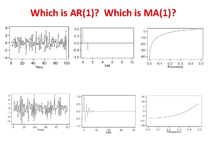
Which is AR(1)? Which is MA(1)?
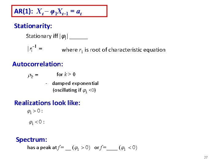
AR(1): X t – φ 1 Xt – 1 = at Stationarity: Stationary iff |j 1| ______ where r 1 is root of characteristic equation Autocorrelation: for k > 0 - damped exponential (oscillating if j 1 <0) Realizations look like: j 1 > 0 j 1 < 0 Spectrum: has a peak at f = __ (j 1 > 0) or f =____ (j 1 < 0) 27
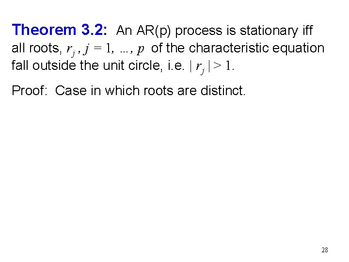
Theorem 3. 2: An AR(p) process is stationary iff all roots, r j , j = 1, …, p of the characteristic equation fall outside the unit circle, i. e. | r j | > 1. Proof: Case in which roots are distinct. 28
29
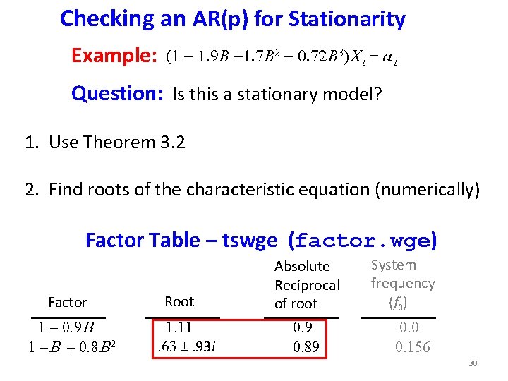
Checking an AR(p) for Stationarity Example: (1 1. 9 B +1. 7 B 2 0. 72 B 3) X t = a t Question: Is this a stationary model? 1. Use Theorem 3. 2 2. Find roots of the characteristic equation (numerically) Factor Table – tswge (factor. wge) Factor 1 0. 9 B 1 B + 0. 8 B 2 Root 1. 11. 63 ±. 93 i Absolute Reciprocal of root 0. 9 0. 89 System frequency (f 0) 0. 0 0. 156 30
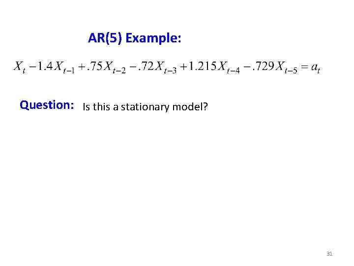
AR(5) Example: Question: Is this a stationary model? 31
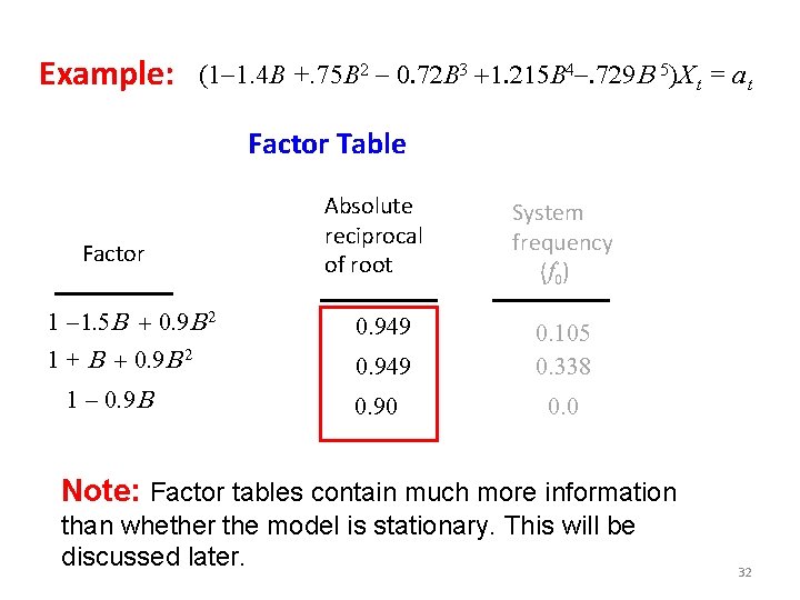
Example: (1 1. 4 B +. 75 B 2 0. 72 B 3 +1. 215 B 4. 729 B 5)X t = a t Factor Table Factor Absolute reciprocal of root System frequency (f 0) 1 1. 5 B + 0. 9 B 2 0. 949 1 + B + 0. 9 B 2 0. 949 0. 105 0. 338 0. 90 0. 0 1 0. 9 B Note: Factor tables contain much more information than whether the model is stationary. This will be discussed later. 32
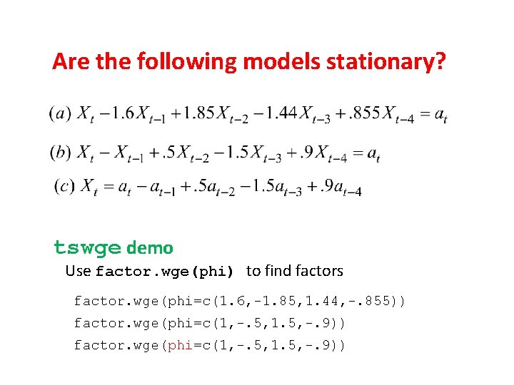
Are the following models stationary? tswge demo Use factor. wge(phi) to find factors factor. wge(phi=c(1. 6, -1. 85, 1. 44, -. 855)) factor. wge(phi=c(1, -. 5, 1. 5, -. 9))
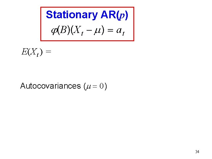
Stationary AR(p) j(B)(X t - m ) = a t E(X t ) = Autocovariances (m = 0 ) 34
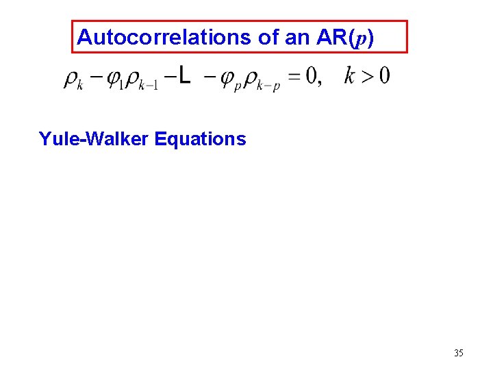
Autocorrelations of an AR(p) Yule-Walker Equations 35
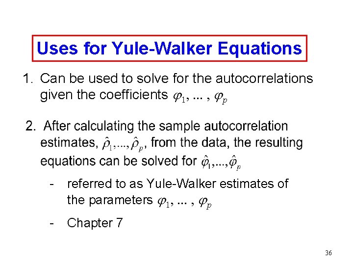
Uses for Yule-Walker Equations 1. Can be used to solve for the autocorrelations given the coefficients j 1, . . . , j p - referred to as Yule-Walker estimates of the parameters j 1, . . . , j p - Chapter 7 36
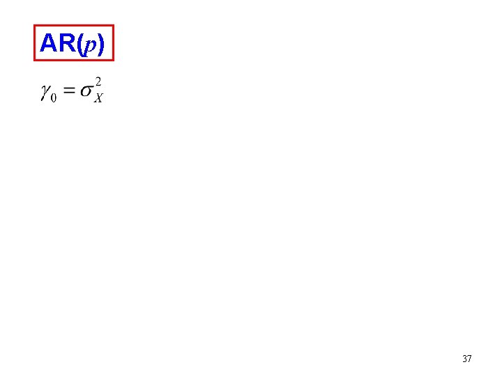
AR(p) 37
AR(p) Spectrum 38
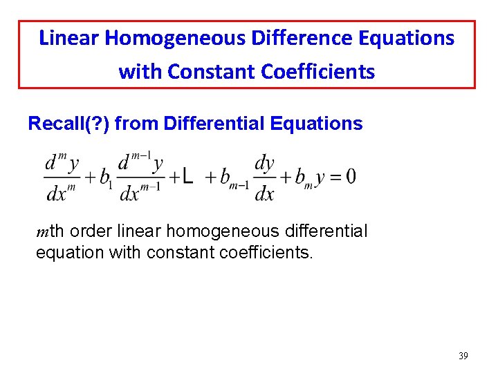
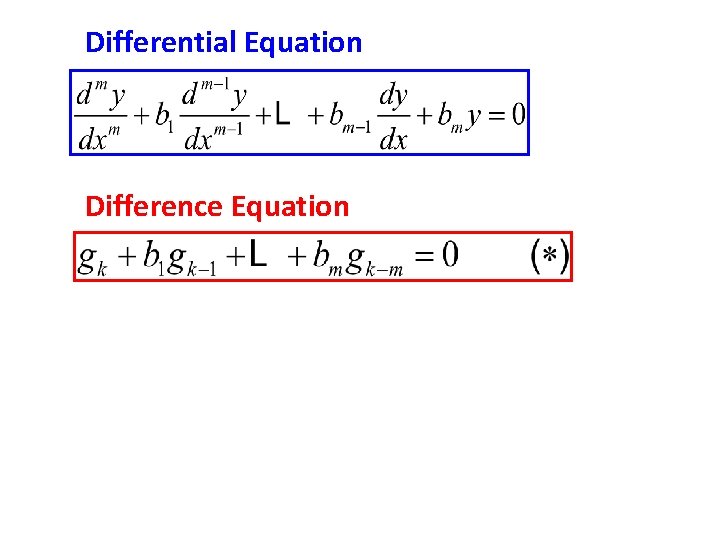
Linear Homogeneous Difference Equations with Constant Coefficients Recall(? ) from Differential Equations m th order linear homogeneous differential equation with constant coefficients. 39
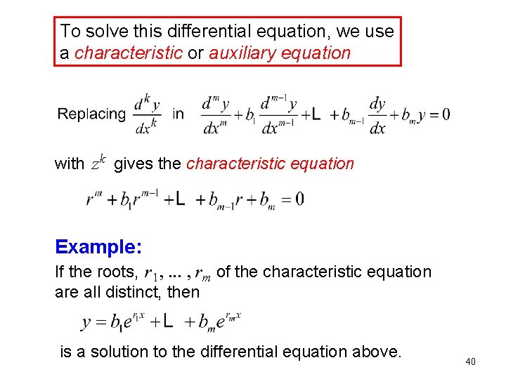
To solve this differential equation, we use a characteristic or auxiliary equation with zk gives the characteristic equation Example: If the roots, r 1, . . . , rm of the characteristic equation are all distinct, then is a solution to the differential equation above. 40
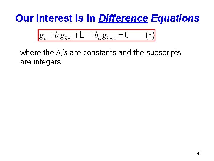
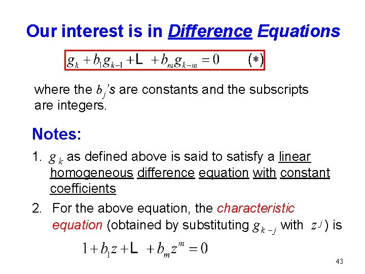
Our interest is in Difference Equations where the b j’s are constants and the subscripts are integers. 41
Differential Equation Difference Equation
Our interest is in Difference Equations where the b j’s are constants and the subscripts are integers. Notes: 1. g k as defined above is said to satisfy a linear homogeneous difference equation with constant coefficients 2. For the above equation, the characteristic equation (obtained by substituting g k - j with z j ) is 43
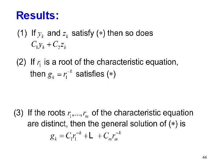
Results: 44
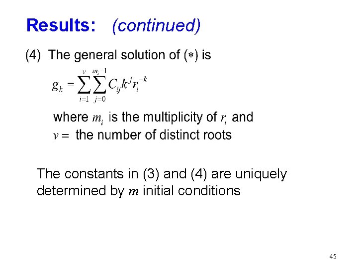
Results: (continued) The constants in (3) and (4) are uniquely determined by m initial conditions 45
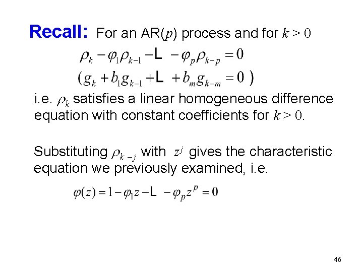
Recall: For an AR(p) process and for k > 0 i. e. r k satisfies a linear homogeneous difference equation with constant coefficients for k > 0. Substituting r k - j with z j gives the characteristic equation we previously examined, i. e. 46
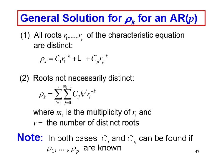
General Solution for r k for an AR(p) Note: In both cases, C i and C ij can be found if r 1, . . . , r p are known 47
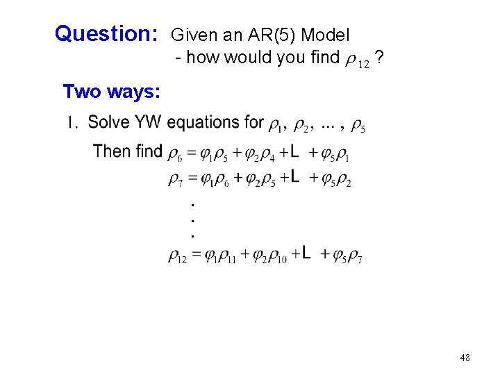
Question: Given an AR(5) Model - how would you find r 12 ? Two ways: . . . 48
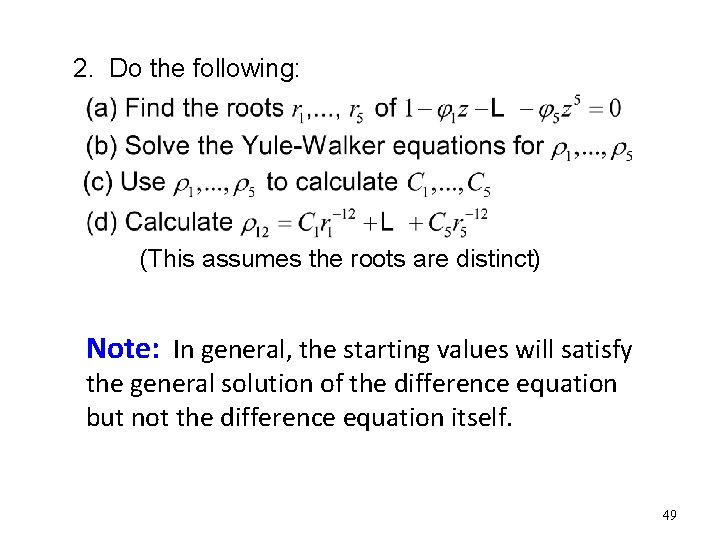
2. Do the following: (This assumes the roots are distinct) Note: In general, the starting values will satisfy the general solution of the difference equation but not the difference equation itself. 49
Recall for AR(1) Models “wandering” realizations” damped exponential autocorrelations spectral density has a peak at f = 0
oscillatory realizations oscillating damped exponential autocorrelations spectral density has a peak at f =. 5
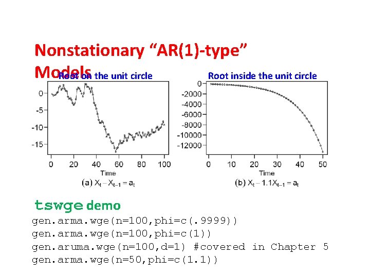
Nonstationary “AR(1)-type” Models Root on the unit circle Root inside the unit circle tswge demo gen. arma. wge(n=100, phi=c(. 9999)) gen. arma. wge(n=100, phi=c(1)) gen. aruma. wge(n=100, d=1) #covered in Chapter 5 gen. arma. wge(n=50, phi=c(1. 1))
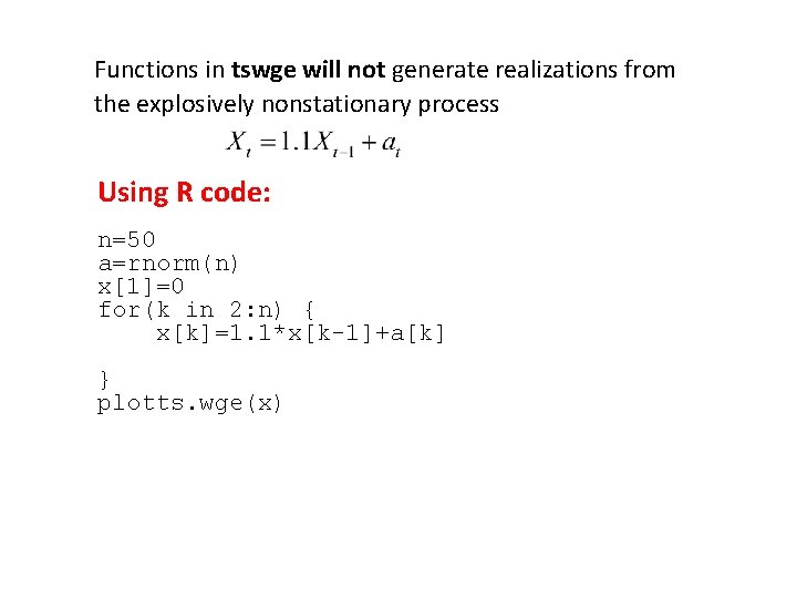
Functions in tswge will not generate realizations from the explosively nonstationary process Using R code: n=50 a=rnorm(n) x[1]=0 for(k in 2: n) { x[k]=1. 1*x[k-1]+a[k] } plotts. wge(x)
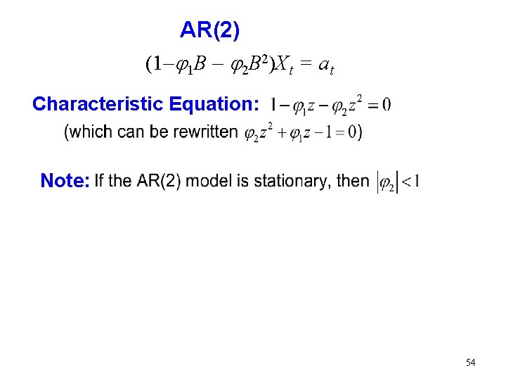
AR(2) (1 j 1 B j 2 B 2)X t = a t Characteristic Equation: Note: 54
Behavior of r k for an AR(2) Question: What does the autocorrelation function look like for an AR(2)? Recall: For an AR(1), r k looks like a “damped exponential” j 1 > 0 (1 j 1 B)X t = a t j 1 < 0 55
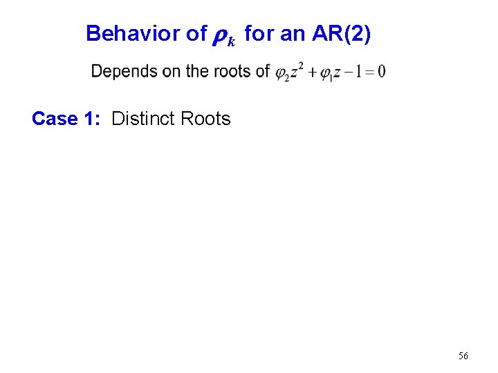
Behavior of r k for an AR(2) Case 1: Distinct Roots 56
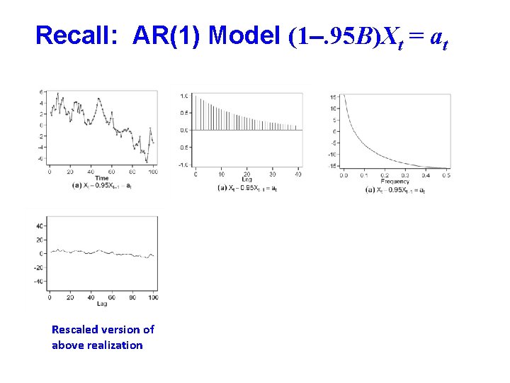
Recall: AR(1) Model (1. 95 B)Xt = at Rescaled version of above realization
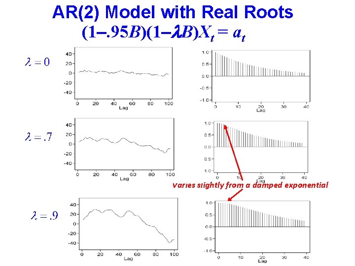
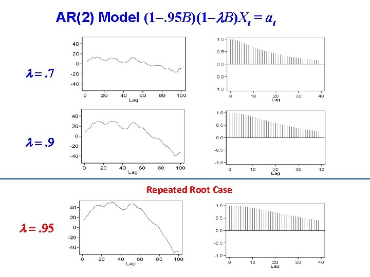
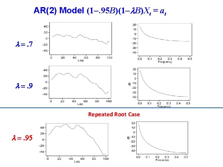
AR(2) Model with Real Roots (1. 95 B)(1 l. B)Xt = at Varies slightly from a damped exponential
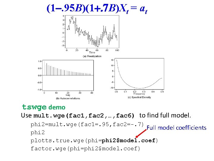
(1. 95 B)(1+. 7 B)Xt = at tswge demo Use mult. wge(fac 1, fac 2, …, fac 6) to find full model. phi 2=mult. wge(fac 1=. 95, fac 2=-. 7) Full model coefficients phi 2 plotts. true. wge(phi=phi 2$model. coef) factor. wge(phi=phi 2$model. coef)
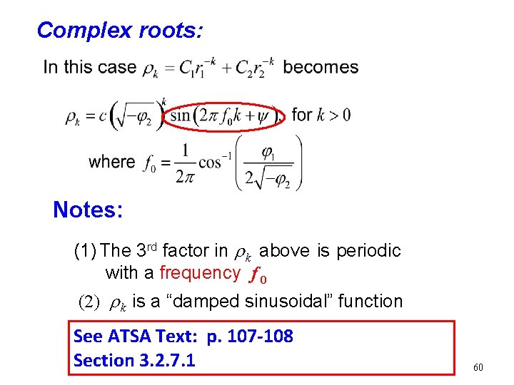
Complex roots: Notes: (1) The 3 rd factor in r k above is periodic with a frequency f 0 (2) r k is a “damped sinusoidal” function See ATSA Text: p. 107 -108 Section 3. 2. 7. 1 60
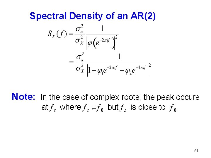
Spectral Density of an AR(2) Note: In the case of complex roots, the peak occurs at f s where f s f 0 but f s is close to f 0 61
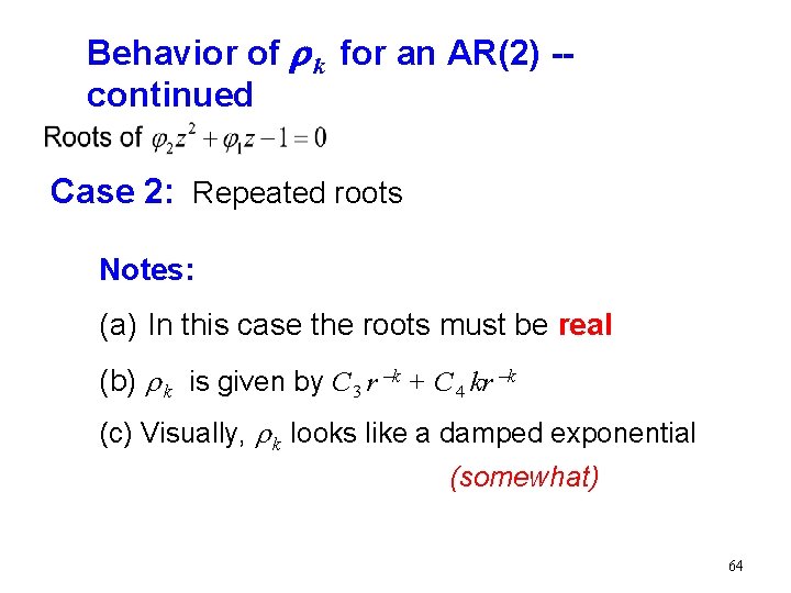
Behavior of r k for an AR(2) -continued Case 2: Repeated roots Notes: (a) In this case the roots must be real (b) r k is given by C 3 r –k + C 4 kr –k (c) Visually, r k looks like a damped exponential (somewhat) 64
AR(2) Model (1. 95 B)(1 l. B)Xt = at l =. 7 l =. 9 Repeated Root Case l =. 95
AR(2) Model (1. 95 B)(1 l. B)Xt = at l =. 7 l =. 9 Repeated Root Case l =. 95
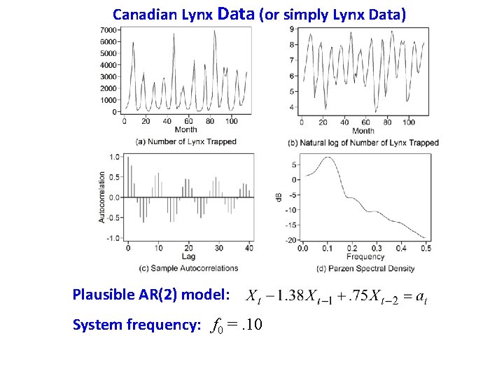
Canadian Lynx Data (or simply Lynx Data) Plausible AR(2) model: System frequency: f 0 =. 10
tswge demo data(llynx) plotts. sample. wge(llynx) # factor. wge(phi=c(1. 38, -. 75)) plotts. true. wge(phi=c(1. 38, -. 75))
Key Concept: The AR(1) and AR(2) serve as “building blocks” of an AR(p) model 69
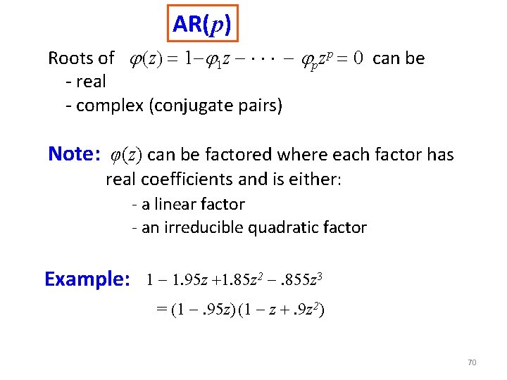
AR( p) Roots of j (z) = 1 j 1 z jpz p = 0 can be - real - complex (conjugate pairs) Note: φ(z) can be factored where each factor has real coefficients and is either: - a linear factor - an irreducible quadratic factor Example: 1 1. 95 z +1. 85 z 2 . 855 z 3 = (1 . 95 z) (1 z +. 9 z 2) 70
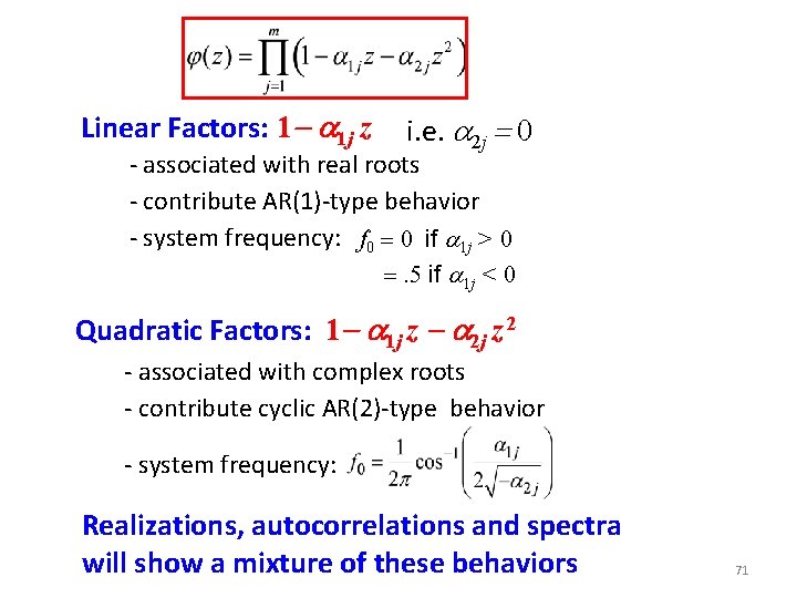
Linear Factors: 1 - a 1 j z i. e. a 2 j = 0 - associated with real roots - contribute AR(1)-type behavior - system frequency: f 0 = 0 if a 1 j > 0 =. 5 if a 1 j < 0 Quadratic Factors: 1 - a 1 j z - a 2 j z 2 - associated with complex roots - contribute cyclic AR(2)-type behavior - system frequency: Realizations, autocorrelations and spectra will show a mixture of these behaviors 71
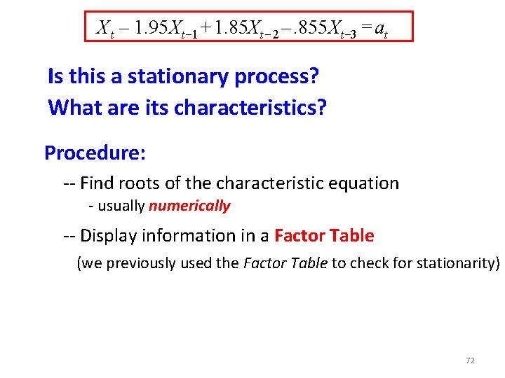
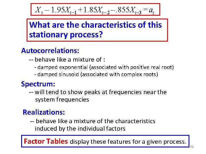
X t – 1. 95 Xt – 1 + 1. 85 Xt – 2 –. 855 Xt – 3 = at Is this a stationary process? What are its characteristics? Procedure: -- Find roots of the characteristic equation - usually numerically -- Display information in a Factor Table (we previously used the Factor Table to check for stationarity) 72
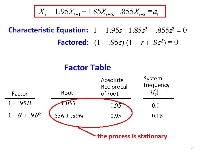
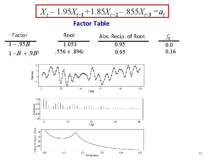
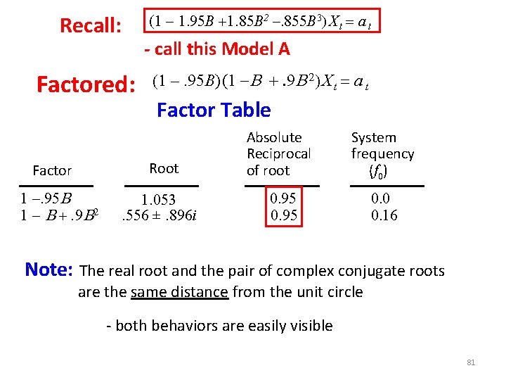
X t – 1. 95 Xt – 1 + 1. 85 Xt – 2 –. 855 Xt – 3 = at Characteristic Equation: 1 1. 95 z +1. 85 z 2 . 855 z 3 = 0 Factored: (1 . 95 z) (1 r +. 9 z 2) = 0 Factor Table System frequency (f 0) Factor Root Absolute Reciprocal of root 1 . 95 B 1. 053 0. 95 0. 0 . 556 ±. 896 i 0. 95 0. 16 1 B +. 9 B 2 the process is stationary 73
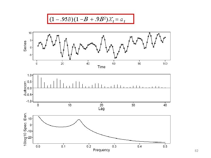
X t – 1. 95 Xt – 1 + 1. 85 Xt – 2 –. 855 Xt – 3 = at What are the characteristics of this stationary process? Autocorrelations: -- behave like a mixture of : - damped exponential (associated with positive real root) - damped sinusoid (associated with complex roots) Spectrum: -- will tend to show peaks at frequencies near the system frequencies Realizations: -- behave like a mixture of the characteristics induced by the individual factors Factor Tables display these features for a given process. 74
X t – 1. 95 Xt – 1 + 1. 85 Xt – 2 –. 855 Xt – 3 = at Factor Table Factor 1 . 95 B 1 B +. 9 B 2 Root 1. 053. 556 ±. 896 i Abs. Recip. of Root 0. 95 f 0 0. 16 75
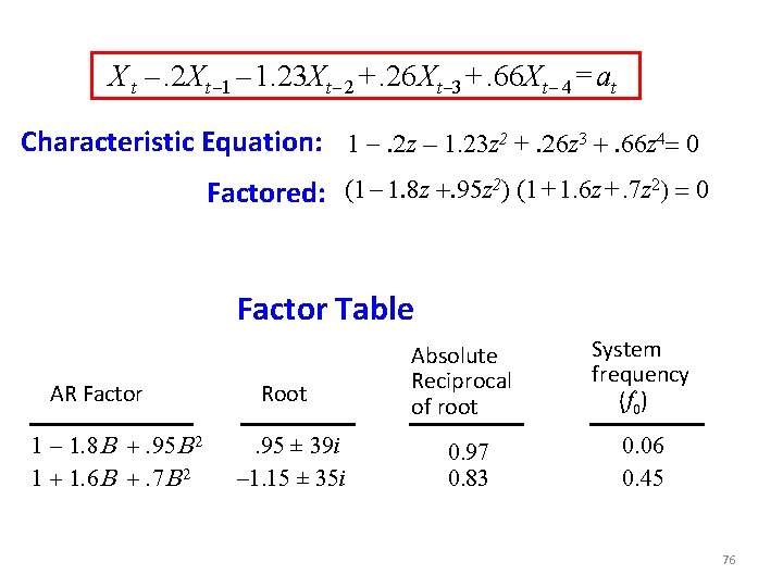
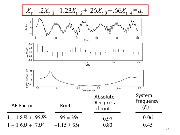
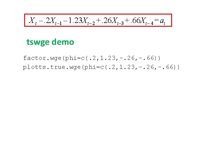
X t –. 2 Xt – 1. 23 Xt – 2 +. 26 Xt – 3 +. 66 Xt – 4 = at Characteristic Equation: 1 . 2 z – 1. 23 z 2 +. 26 z 3 +. 66 z 4= 0 Factored: (1 1. 8 z +. 95 z 2) (1 + 1. 6 z +. 7 z 2) = 0 Factor Table AR Factor 1 1. 8 B +. 95 B 2 1 + 1. 6 B +. 7 B 2 Root. 95 ± 39 i – 1. 15 ± 35 i Absolute Reciprocal of root System frequency (f 0) 0. 97 0. 83 0. 06 0. 45 76
X t –. 2 Xt – 1. 23 Xt – 2 +. 26 Xt – 3 +. 66 Xt – 4 = at AR Factor 1 1. 8 B +. 95 B 2 1 + 1. 6 B +. 7 B 2 Root. 95 ± 39 i – 1. 15 ± 35 i Absolute Reciprocal of root System frequency (f 0) 0. 97 0. 83 0. 06 0. 45 77
X t –. 2 Xt – 1. 23 Xt – 2 +. 26 Xt – 3 +. 66 Xt – 4 = at tswge demo factor. wge(phi=c(. 2, 1. 23, -. 26, -. 66)) plotts. true. wge(phi=c(. 2, 1. 23, -. 26, -. 66))
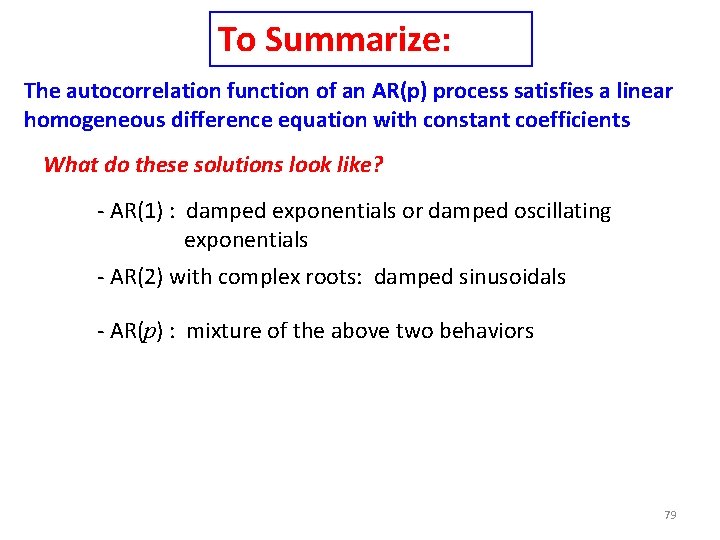
To Summarize: The autocorrelation function of an AR(p) process satisfies a linear homogeneous difference equation with constant coefficients What do these solutions look like? - AR(1) : damped exponentials or damped oscillating exponentials - AR(2) with complex roots: damped sinusoidals - AR(p) : mixture of the above two behaviors 79
General Solution for r k for an AR(p) 80
(1 1. 95 B +1. 85 B 2 –. 855 B 3) X t = a t Recall: - call this Model A Factored: (1 –. 95 B) (1 B +. 9 B 2) X t = a t Factor Table Root Factor 1 . 95 B 1 B +. 9 B 2 1. 053. 556 ±. 896 i Absolute Reciprocal of root System frequency (f 0) 0. 95 0. 0 0. 16 Note: The real root and the pair of complex conjugate roots are the same distance from the unit circle - both behaviors are easily visible 81
(1 –. 95 B) (1 B +. 9 B 2) X t = a t 82
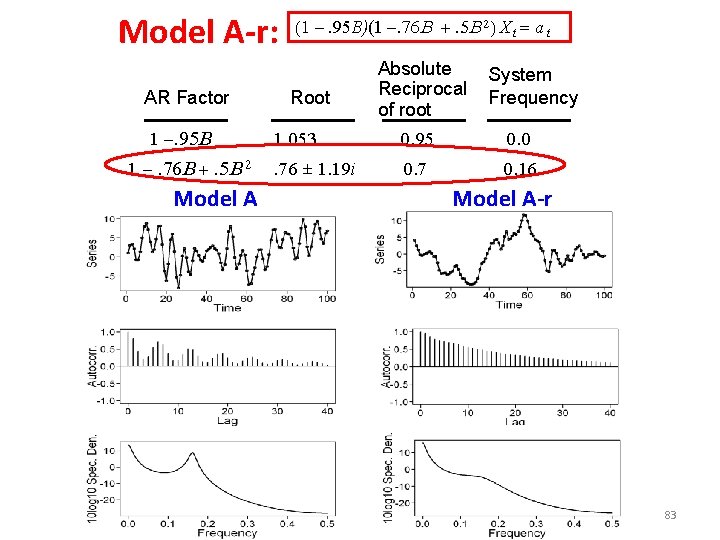
Model A-r: AR Factor 1 . 95 B 1 . 76 B +. 5 B 2 Model A (1 –. 95 B)(1 . 76 B +. 5 B 2) X t = a t Root Absolute Reciprocal of root System Frequency 1. 053 0. 95 0. 0 . 76 ± 1. 19 i 0. 7 0. 16 Model A-r 83
Note: If the root of the first order factor is much closer to the unit circle, -- the first order factor dominates -- the behavior of the autocorrelations (and the realization) becomes “first-order like” – i. e. damped exponentials 84
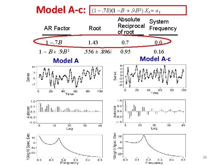
Model A-c: (1 –. 7 B)(1 B +. 9 B 2) X t = a t AR Factor Root 1 . 7 B 1. 43 1 B +. 9 B 2 Model A . 556 ±. 896 i Absolute System Reciprocal Frequency of root 0. 7 0. 0 0. 95 0. 16 Model A-c 85
When roots of the second order factor are much closer to the unit circle, the second order factor dominates -- the behavior of the autocorrelations behave more like a damped sinusoidal which is characteristic of a second order model -- realizations appear more “pseudo-sinusoidal” General Property Roots closest to the unit circle dominate the behavior of autocorrelation functions, realizations, and spectral densities 86
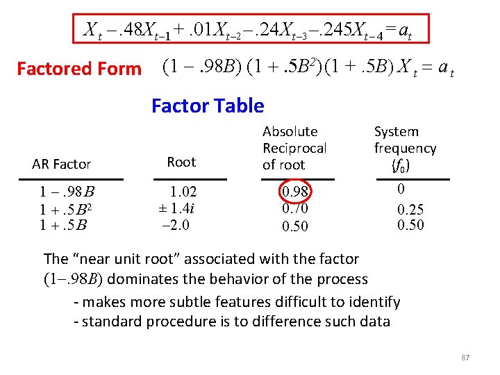
X t –. 48 Xt – 1 +. 01 Xt – 2 –. 24 Xt – 3 –. 245 Xt – 4 = at Factored Form (1 . 98 B) (1 +. 5 B 2) (1 +. 5 B) X t = a t Factor Table AR Factor Root Absolute Reciprocal of root 1 . 98 B 1 +. 5 B 2 1 +. 5 B 1. 02 ± 1. 4 i – 2. 0 0. 98 0. 70 0. 50 System frequency (f 0) 0 0. 25 0. 50 The “near unit root” associated with the factor (1. 98 B) dominates the behavior of the process - makes more subtle features difficult to identify - standard procedure is to difference such data 87
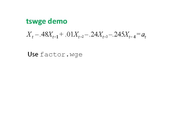
tswge demo X t –. 48 Xt – 1 +. 01 Xt – 2 –. 24 Xt – 3 –. 245 Xt – 4 = at Use factor. wge
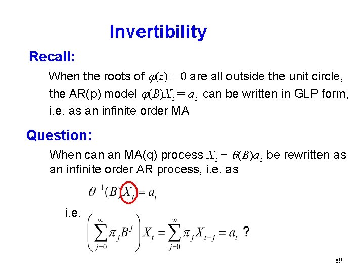
Invertibility Recall: When the roots of j(z) = 0 are all outside the unit circle, the AR(p) model j(B)X t = a t can be written in GLP form, i. e. as an infinite order MA Question: When can an MA(q) process X t = (B)a t be rewritten as an infinite order AR process, i. e. as i. e. 89
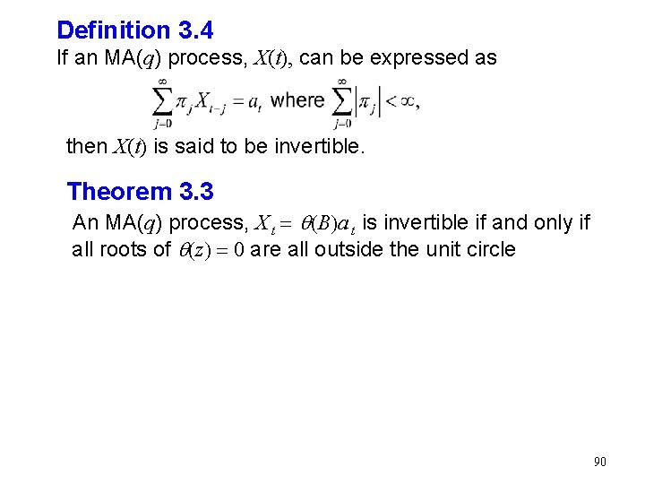
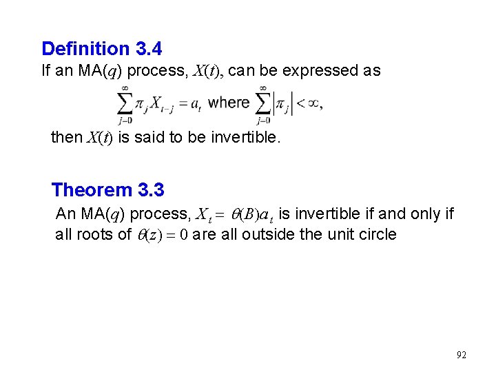
Definition 3. 4 If an MA(q) process, X(t), can be expressed as then X(t) is said to be invertible. Theorem 3. 3 An MA(q) process, X t = (B)a t is invertible if and only if all roots of (z) = 0 are all outside the unit circle 90
Invertibility Example: MA(1) 91
Definition 3. 4 If an MA(q) process, X(t), can be expressed as then X(t) is said to be invertible. Theorem 3. 3 An MA(q) process, X t = (B)a t is invertible if and only if all roots of (z) = 0 are all outside the unit circle 92
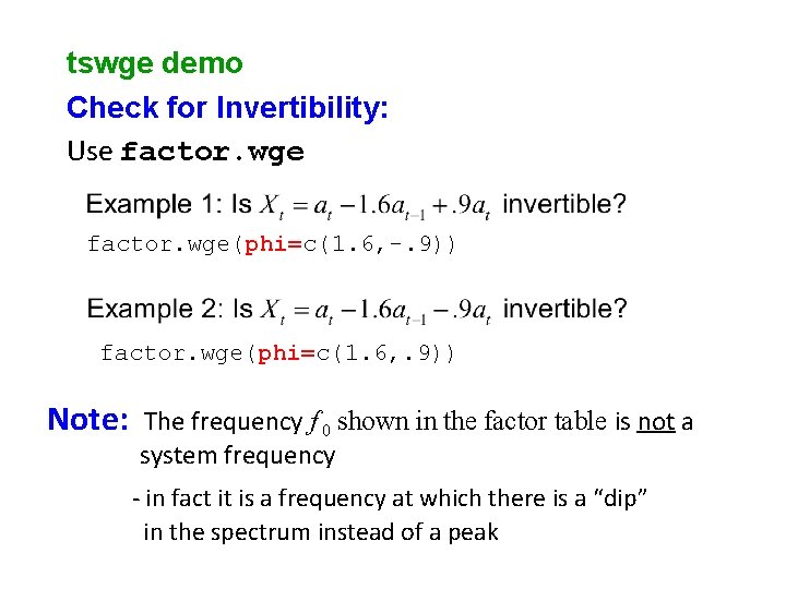
tswge demo Check for Invertibility: Use factor. wge(phi=c(1. 6, -. 9)) factor. wge(phi=c(1. 6, . 9)) Note: The frequency f 0 shown in the factor table is not a system frequency - in fact it is a frequency at which there is a “dip” in the spectrum instead of a peak
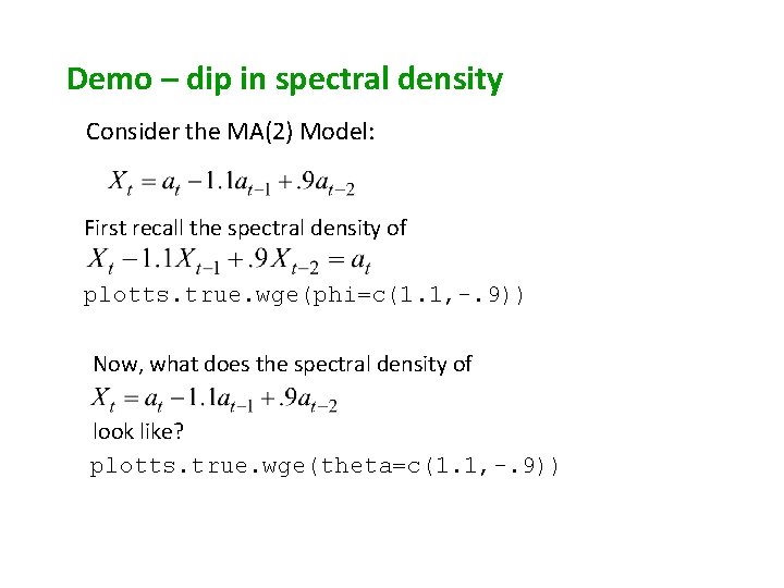
Demo – dip in spectral density Consider the MA(2) Model: First recall the spectral density of plotts. true. wge(phi=c(1. 1, -. 9)) Now, what does the spectral density of look like? plotts. true. wge(theta=c(1. 1, -. 9))
Why worry about invertibility? 1. Invertibility assures that the present is related to the past in a reasonable manner. 2. Removes model multiplicity 95
tswge demo 1. X t = at –. 9 at – 1 2. X t = at – 1. 111 at – 1 Note: 1/. 9 = 1. 1111…. Use plotts. true. wge to compare the characteristics of these two models 96
Summary MA(q) Process: • always stationary ( if | i |’s < ) • invertible if and only if the roots of (z) = 0 lie outside the unit circle AR(p) Process: • stationary if and only if the roots of j (z) = 0 lie outside the unit circle • always invertible ( if | j i |’s < ) In general, we will restrict our attention to stationary and invertible models. 97
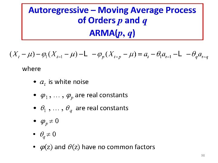
Autoregressive – Moving Average Process of Orders p and q ARMA(p, q) where • a t is white noise • j 1 , … , j p are real constants • 1 , … , q are real constants • jp 0 • q 0 • j (z) and (z) have no common factors 98
Notes: 1. I will typically use the “zero mean” form of the model 2. Operator Notation: 99
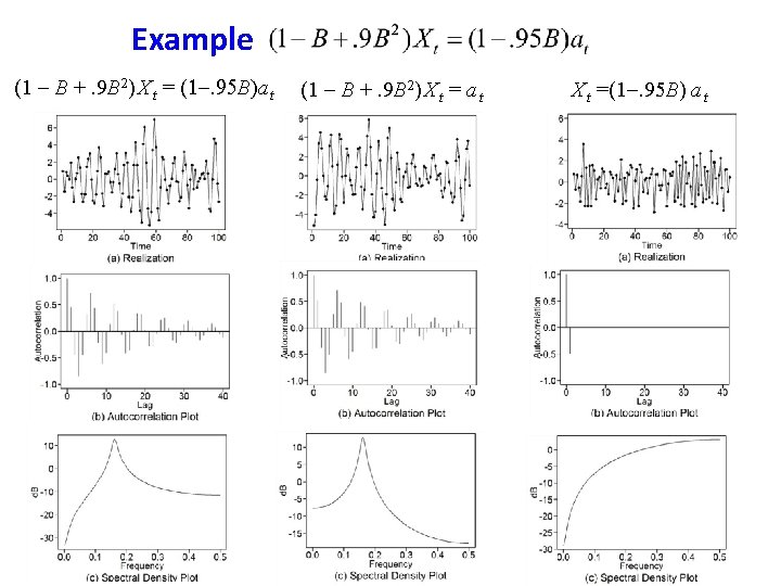
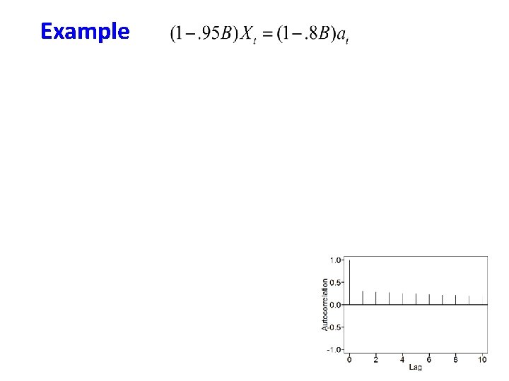
Example (1 B +. 9 B 2) X t = (1. 95 B)a t (1 B +. 9 B 2) X t = a t X t =(1. 95 B) a t
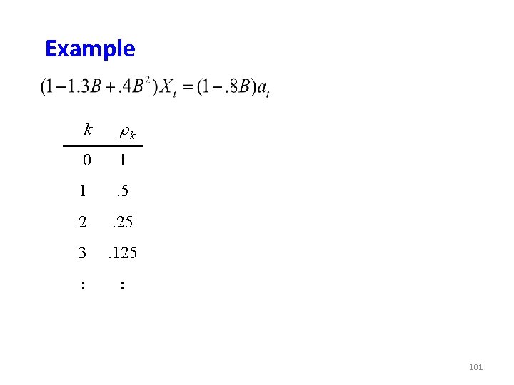
Example k rk 0 1 1 . 5 2 . 25 3 . 125 101
ARMA(p, q) Model j (B )X t = q (B )a t • j (B ) and (B ) introduce characteristics of the same type as in the AR(p) and MA(q) cases • “near cancellation” may “hide” some characteristics Theorem 3. 4: Let X t be a causal process specified by j (B)X t = (B)a t. Then X t is an ARMA(p, q) process iff (i) roots of j (z) = 0 are all outside the unit circle (ii) roots of (z) = 0 are all outside the unit circle 102
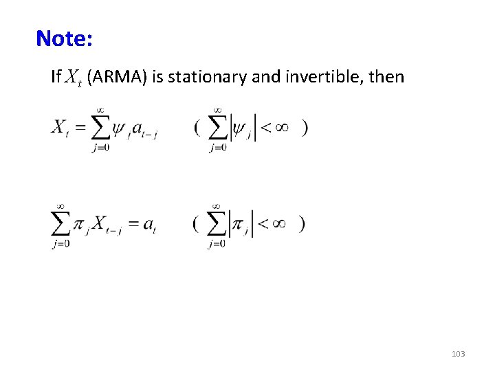
Note: If X t (ARMA) is stationary and invertible, then 103
Autocovariances and Autocorrelations of an ARMA(p, q) 104
Calculating Autocovariance, g. K, for an ARMA(p, q) Model 1. Solve (v+1) x (v+1) system of equations for go, . . . , g v where v = max(p, q) 2. Two ways to proceed beyond step 1: (a) calculate g K by recursively calculating g k = j 1 g k-1 + + jpg k-p until we reach K (b) since g k satisfies a linear homogeneous difference equation for k > q, use the general solution to solve for g K 105
Example 106
ARMA (p, q) Spectral Density 107
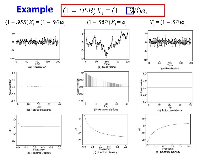
Example (1 –. 95 B) X t = (1 . 9 B)a t (1 –. 95 B) X t = a t X t = (1 . 9 B)a t 108
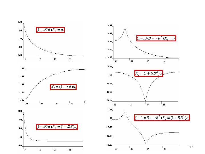
109
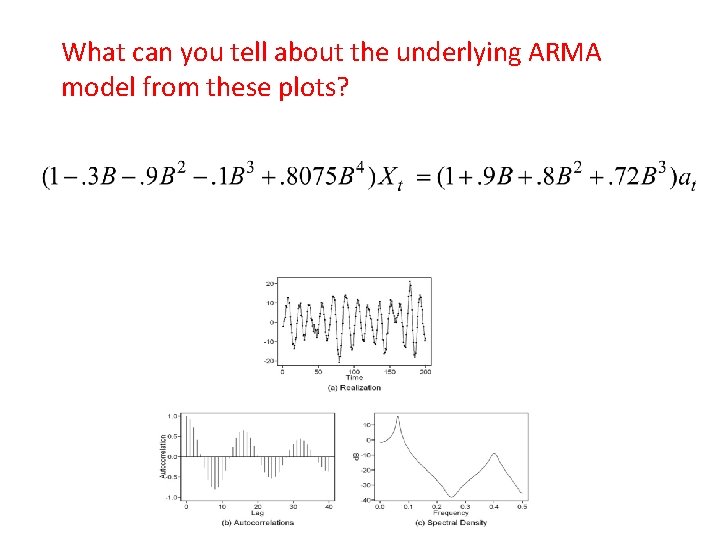
What can you tell about the underlying ARMA model from these plots?
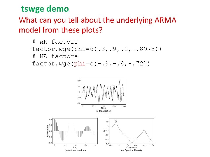
tswge demo What can you tell about the underlying ARMA model from these plots? # AR factors factor. wge(phi=c(. 3, . 9, . 1, -. 8075)) # MA factors factor. wge(phi=c(-. 9, -. 8, -. 72))
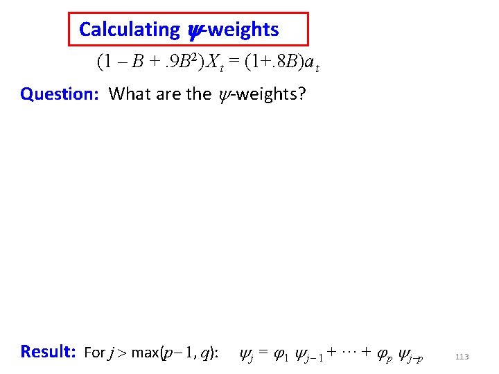
Calculating y-weights (1 – B +. 9 B 2) X t = (1+. 8 B)a t Question: What are the y-weights? 3 methods discussed in book (Chapter 3, pages 144 -146) (a) Equating coefficients (b) Using division (c) General expression Result: For j > max(p 1, q): y j = j 1 y j- 1 + ··· + j p y j-p 112
Calculating y-weights (1 – B +. 9 B 2) X t = (1+. 8 B)a t Question: What are the y-weights? Result: For j > max(p 1, q): y j = j 1 y j- 1 + ··· + j p y j-p 113
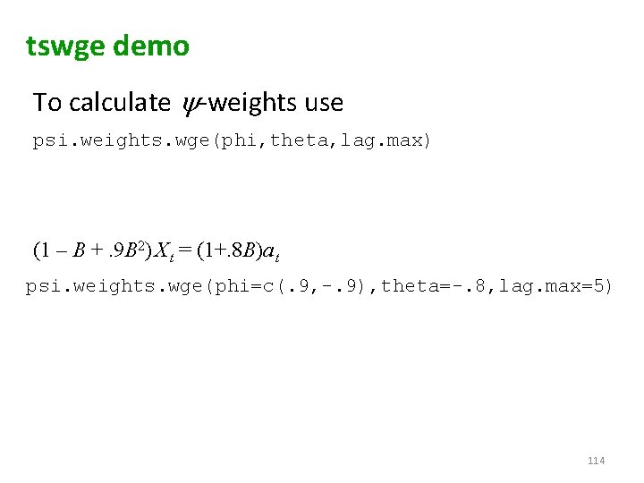
tswge demo To calculate y-weights use psi. weights. wge(phi, theta, lag. max) (1 – B +. 9 B 2) X t = (1+. 8 B)a t psi. weights. wge(phi=c(. 9, -. 9), theta=-. 8, lag. max=5) 114
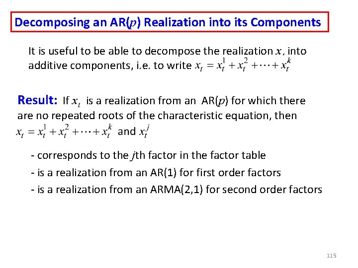
Decomposing an AR(p) Realization into its Components It is useful to be able to decompose the realization x t into additive components, i. e. to write Result: If x t is a realization from an AR(p) for which there are no repeated roots of the characteristic equation, then - corresponds to the jth factor in the factor table - is a realization from an AR(1) for first order factors - is a realization from an ARMA(2, 1) for second order factors 115
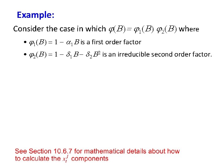
Example: Consider the case in which j(B ) = j 1(B ) j 2(B ) where • j 1(B ) = 1 a 1 B is a first order factor • j 2(B ) = 1 d 1 B d 2 B 2 is an irreducible second order factor.
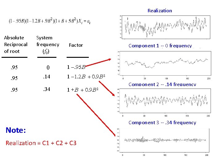
Realization Absolute Reciprocal of root System frequency (f 0) Factor . 95 0 1 . 95 B . 95 . 14 . 95 . 34 Component 1 -- 0 frequency 1 1. 2 B + 0. 9 B 2 1 +B + 0. 9 B 2 Note: Component 2 --. 14 frequency Component 3 --. 34 frequency Realization = C 1 + C 2 + C 3 117
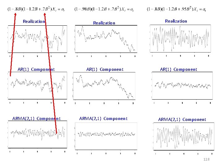
Realization AR(1) Component ARMA(2, 1) Component 118
Decomposition of an AR Process into its Additive Components The important points to be understood are that: (1) each component corresponds to a row in the factor table (2) the components add to give Xt , i. e the components provide a visual representation for the information in the factor table. 119
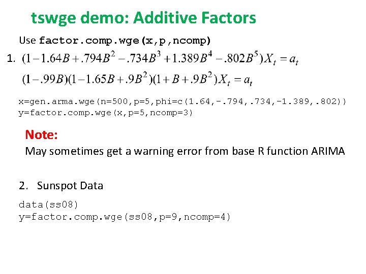
tswge demo: Additive Factors Use factor. comp. wge(x, p, ncomp) 1. x=gen. arma. wge(n=500, p=5, phi=c(1. 64, -. 794, . 734, -1. 389, . 802)) y=factor. comp. wge(x, p=5, ncomp=3) Note: May sometimes get a warning error from base R function ARIMA 2. Sunspot Data data(ss 08) y=factor. comp. wge(ss 08, p=9, ncomp=4)
Seasonal Models - most important seasonal models are nonstationary - we will discuss these in Chapter 5
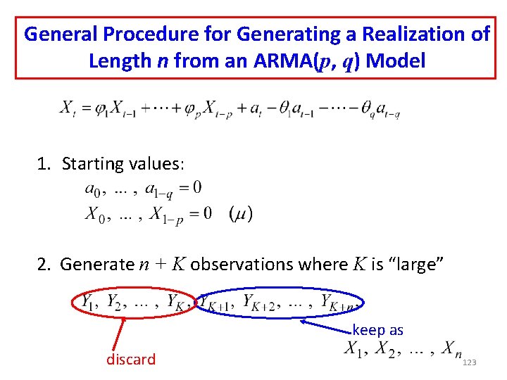
Generating Realizations from an ARMA (p, q) Process MA(q) AR(p) 122
General Procedure for Generating a Realization of Length n from an ARMA(p, q) Model 1. Starting values: 2. Generate n + K observations where K is “large” keep as discard 123
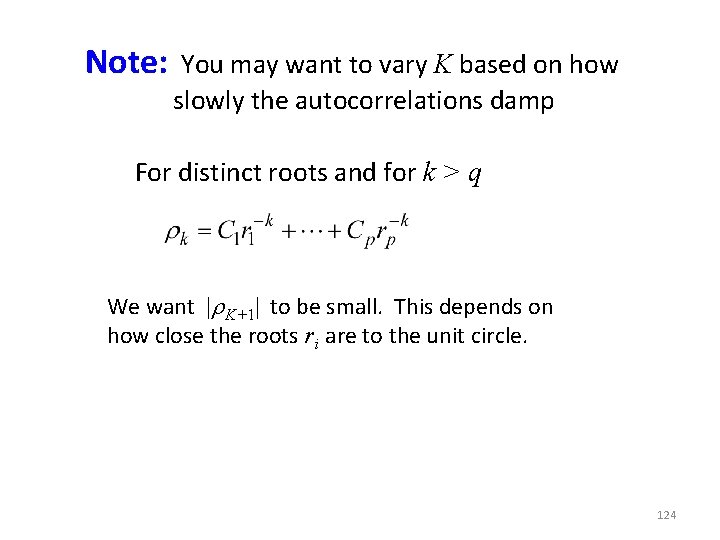
Note: You may want to vary K based on how slowly the autocorrelations damp For distinct roots and for k > q We want |r K+1| to be small. This depends on how close the roots r i are to the unit circle. 124
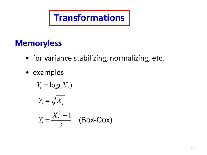
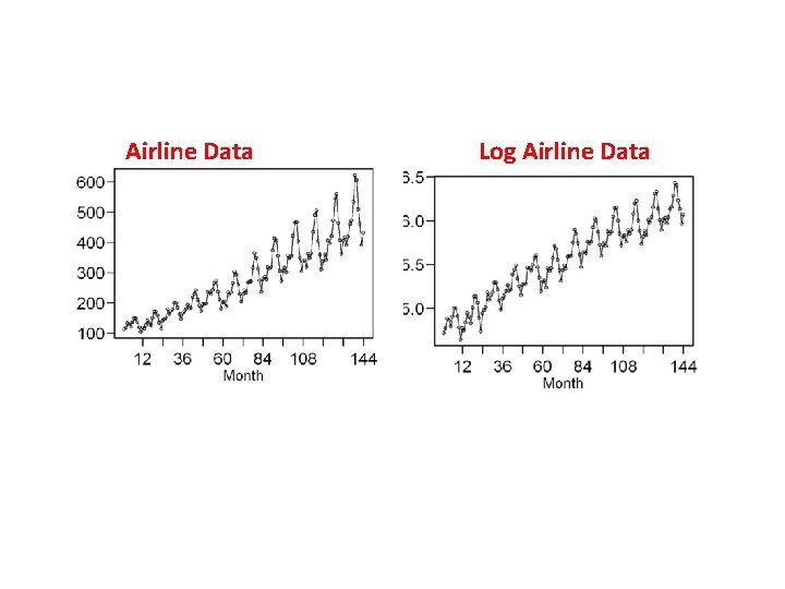
Transformations Memoryless • for variance stabilizing, normalizing, etc. • examples 125
Airline Data Log Airline Data
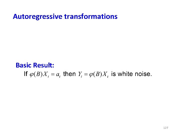
Autoregressive transformations Basic Result: 127
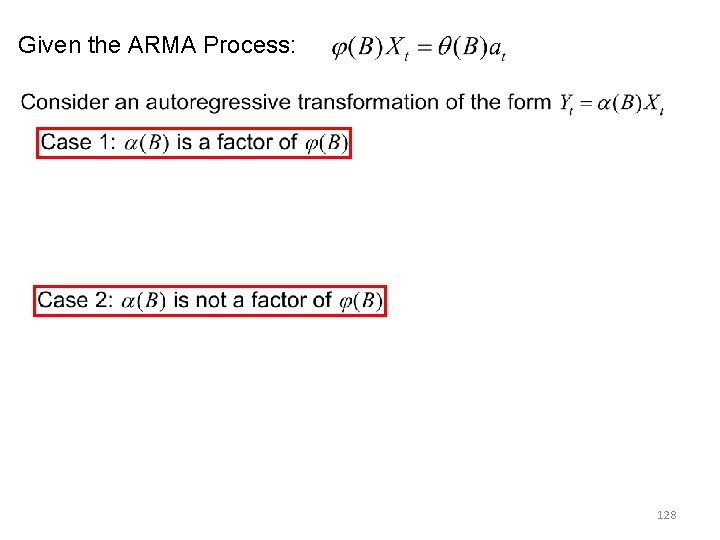
Given the ARMA Process: 128
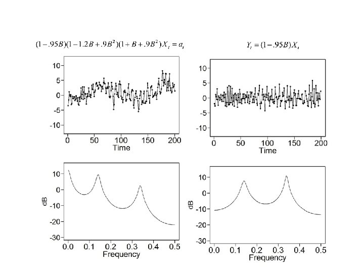
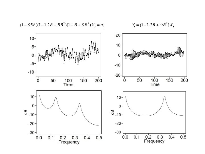
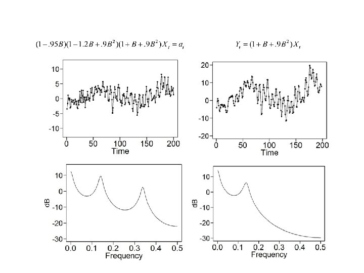
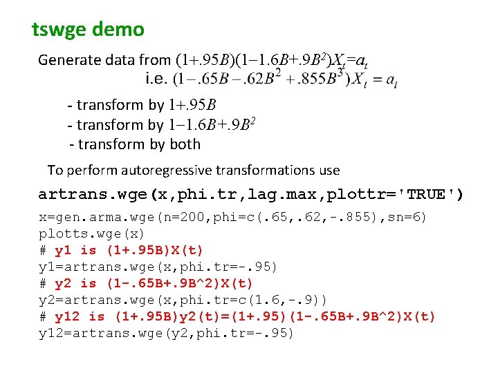
tswge demo Generate data from (1+. 95 B)(1 1. 6 B+. 9 B 2)Xt=at - transform by 1+. 95 B - transform by 1 1. 6 B+. 9 B 2 - transform by both To perform autoregressive transformations use artrans. wge(x, phi. tr, lag. max, plottr='TRUE') x=gen. arma. wge(n=200, phi=c(. 65, . 62, -. 855), sn=6) plotts. wge(x) # y 1 is (1+. 95 B)X(t) y 1=artrans. wge(x, phi. tr=-. 95) # y 2 is (1 -. 65 B+. 9 B^2)X(t) y 2=artrans. wge(x, phi. tr=c(1. 6, -. 9)) # y 12 is (1+. 95 B)y 2(t)=(1+. 95)(1 -. 65 B+. 9 B^2)X(t) y 12=artrans. wge(y 2, phi. tr=-. 95)
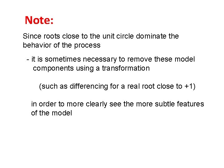
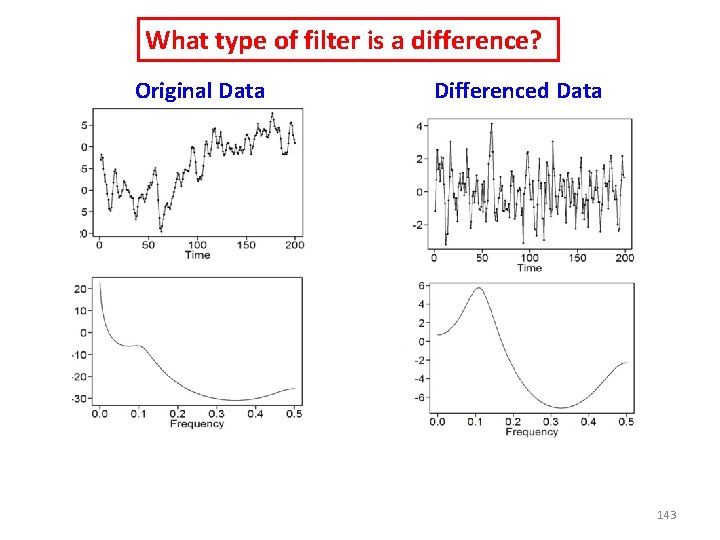
Note: Since roots close to the unit circle dominate the behavior of the process - it is sometimes necessary to remove these model components using a transformation (such as differencing for a real root close to +1) in order to more clearly see the more subtle features of the model
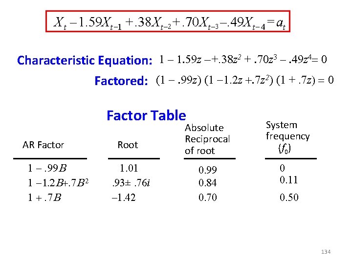
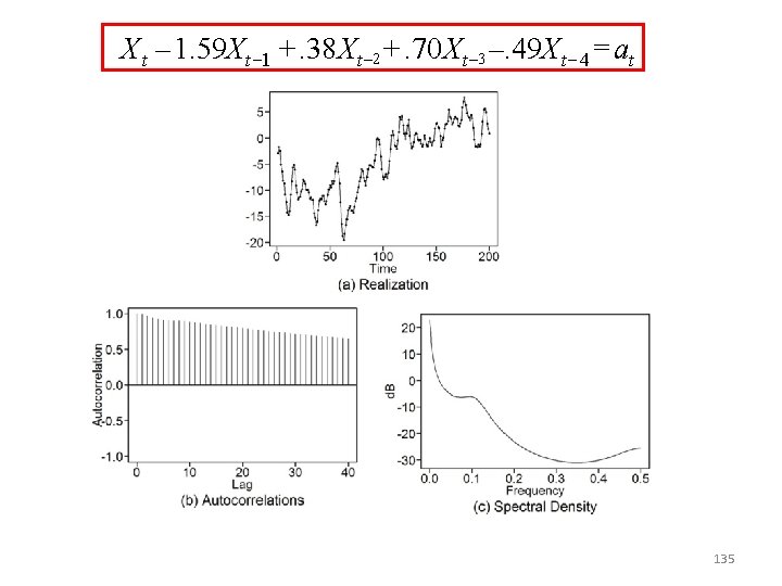
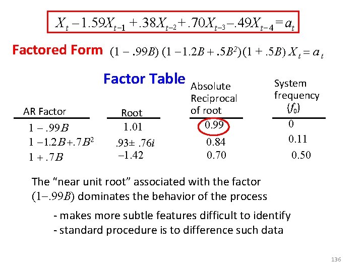
X t – 1. 59 Xt – 1 +. 38 Xt – 2 +. 70 Xt – 3 –. 49 Xt – 4 = at Characteristic Equation: 1 – 1. 59 z –+. 38 z 2 +. 70 z 3 –. 49 z 4= 0 Factored: (1 . 99 z) (1 1. 2 z +. 7 z 2) (1 +. 7 z) = 0 Factor Table AR Factor 1 . 99 B 1 1. 2 B+. 7 B 2 1 +. 7 B Root 1. 01. 93±. 76 i – 1. 42 Absolute Reciprocal of root System frequency (f 0) 0. 99 0. 84 0. 70 0 0. 11 0. 50 134
X t – 1. 59 Xt – 1 +. 38 Xt – 2 +. 70 Xt – 3 –. 49 Xt – 4 = at 135
X t – 1. 59 Xt – 1 +. 38 Xt – 2 +. 70 Xt – 3 –. 49 Xt – 4 = at Factored Form (1 . 99 B) (1 1. 2 B +. 5 B 2) (1 +. 5 B) X t = a t Factor Table AR Factor 1 . 99 B 1 1. 2 B +. 7 B 2 1 +. 7 B Root 1. 01. 93±. 76 i – 1. 42 Absolute Reciprocal of root 0. 99 0. 84 0. 70 System frequency (f 0) 0 0. 11 0. 50 The “near unit root” associated with the factor (1. 99 B) dominates the behavior of the process - makes more subtle features difficult to identify - standard procedure is to difference such data 136
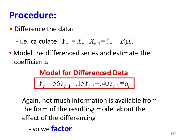
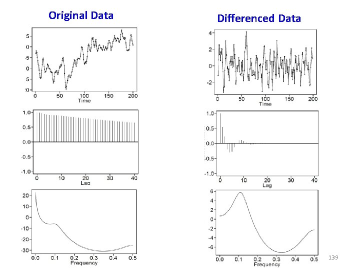
Procedure: • Difference the data: - i. e. calculate Y t = X t – Xt – 1= (1 − B)Xt • Model the differenced series and estimate the coefficients Model for Differenced Data Y t . 56 Yt – 1 . 15 Yt – 2 +. 40 Yt – 3 = at Again, not much information is available from the form of the resulting model about the effect of the differencing - so we factor 137
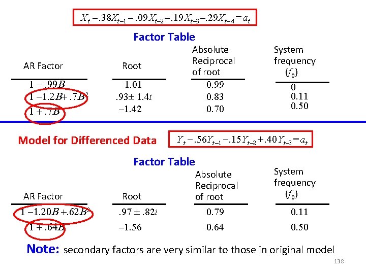
X t –. 38 Xt – 1 –. 09 Xt – 2 –. 19 Xt – 3 –. 29 Xt – 4 = at Factor Table AR Factor 1 . 99 B 1 1. 2 B+. 7 B 2 1 +. 7 B Root 1. 01. 93± 1. 4 i – 1. 42 Model for Differenced Data Absolute Reciprocal of root 0. 99 0. 83 0. 70 1 1. 20 B +. 62 B 2 1 +. 64 B Root. 97 ±. 82 i – 1. 56 0 0. 11 0. 50 Y t . 56 Yt – 1 . 15 Yt – 2 +. 40 Yt – 3 = at Factor Table AR Factor System frequency (f 0) Absolute Reciprocal of root 0. 79 0. 64 System frequency (f 0) 0. 11 0. 50 Note: secondary factors are very similar to those in original model 138
Original Data Differenced Data 139
Note: Differencing can be used to remove the effects of a factor close to 1 B - this topic is discussed further in Chapters 5, 8, and 9 tswge demo To apply a difference filter to data set x use artrans. wge(x, phi=1)
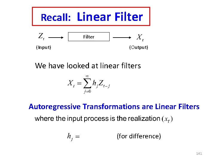
Recall: Linear Filter (Input) (Output) We have looked at linear filters Autoregressive Transformations are Linear Filters (for difference) 141
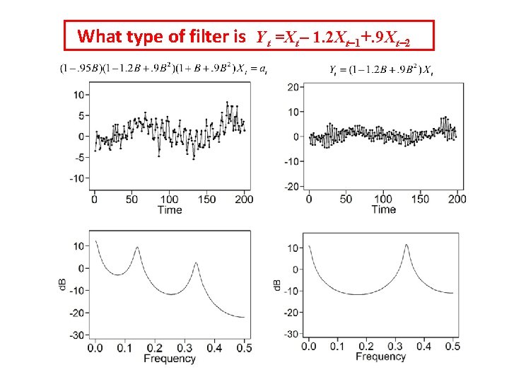
Types of Filters Low-pass filters: - “pass” low frequency behavior and “filter out” higher frequency behavior High-pass filters: - “pass” high frequency behavior and “filter out” lower frequency behavior Band-pass filters: - “pass” frequencies in a certain “frequency band” Band-stop (notch) filters: - “pass” frequencies except those in a certain “frequency band” 142
What type of filter is a difference? Original Data Differenced Data 143
What type of filter is Y t =Xt – 1. 2 Xt 1 +. 9 Xt-2