Taking a model to the computer Martin Ellison
- Slides: 24

Taking a model to the computer Martin Ellison University of Warwick and CEPR Bank of England, December 2005

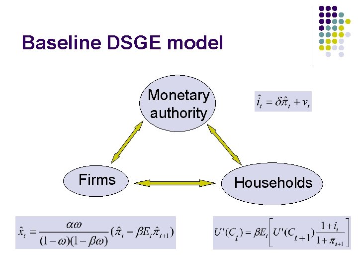
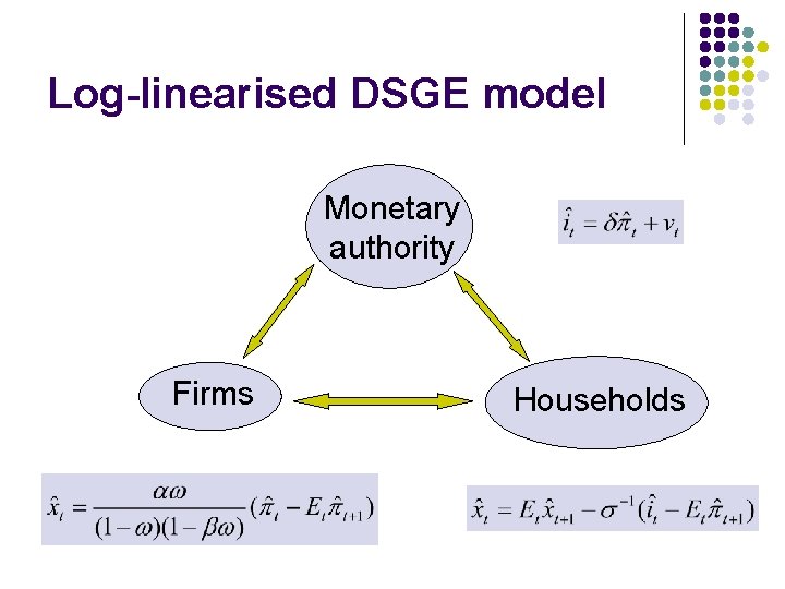
Baseline DSGE model Monetary authority Firms Households

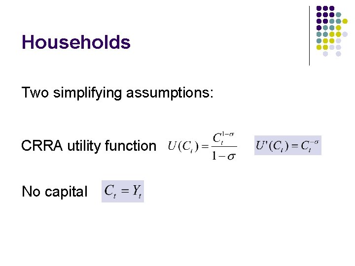
Households Two simplifying assumptions: CRRA utility function No capital

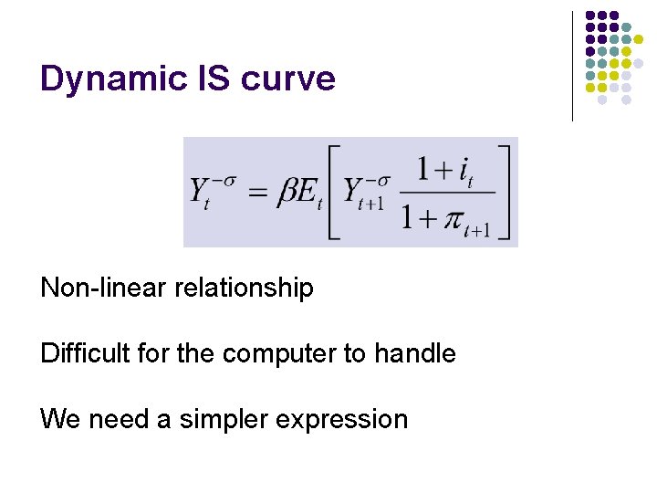
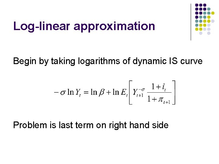
Dynamic IS curve Non-linear relationship Difficult for the computer to handle We need a simpler expression

Log-linear approximation Begin by taking logarithms of dynamic IS curve Problem is last term on right hand side

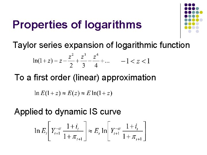
Properties of logarithms Taylor series expansion of logarithmic function To a first order (linear) approximation Applied to dynamic IS curve

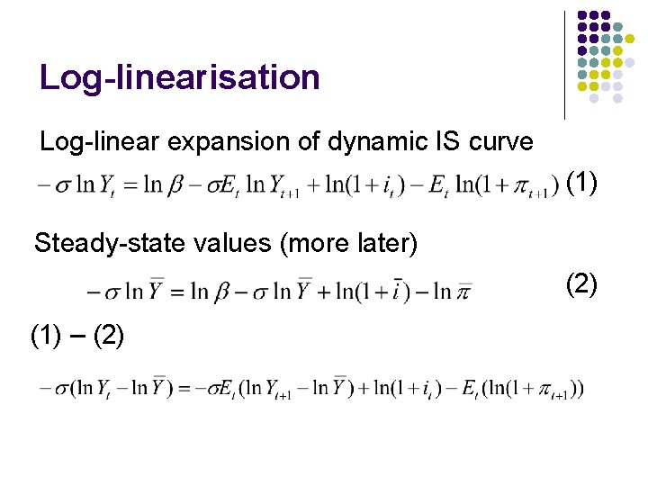
Log-linearisation Log-linear expansion of dynamic IS curve (1) Steady-state values (more later) (2) (1) – (2)

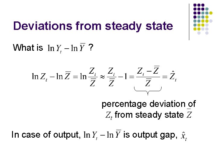
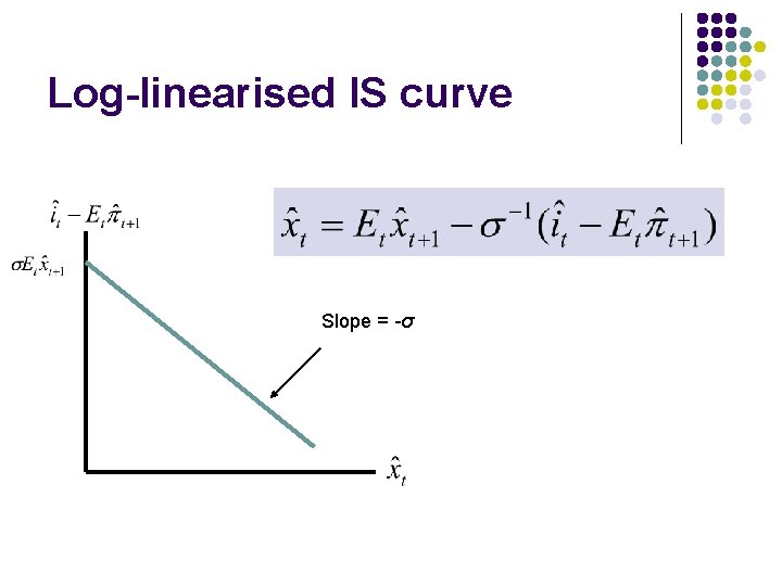
Deviations from steady state What is ? percentage deviation of Zt from steady state Z In case of output, is output gap,

Log-linearised IS curve Slope = -σ

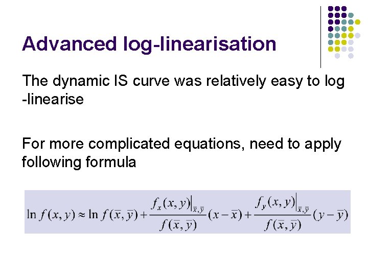
Advanced log-linearisation The dynamic IS curve was relatively easy to log -linearise For more complicated equations, need to apply following formula

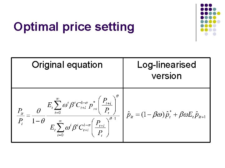
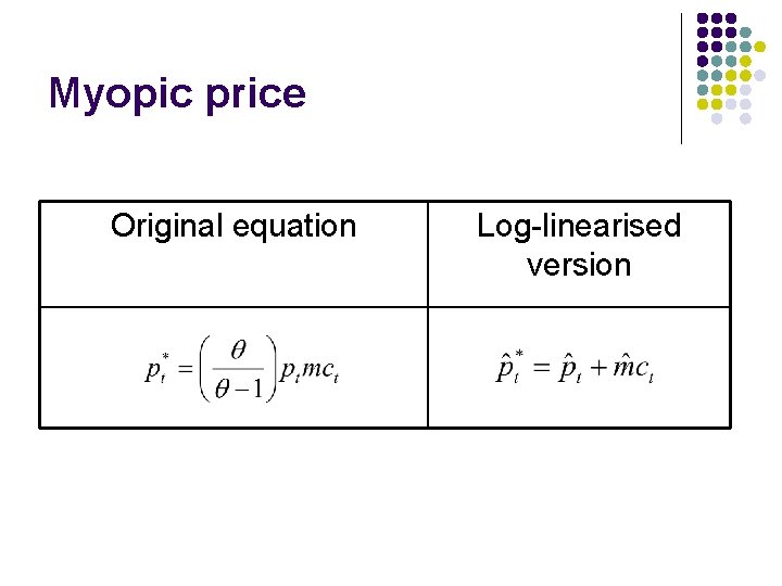
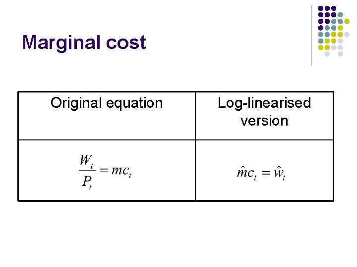
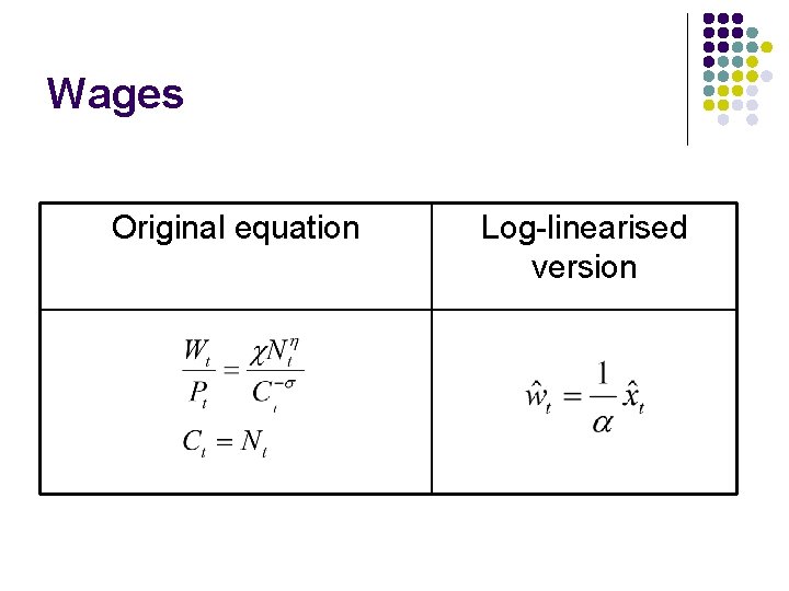
Firms Previously solved for firm behaviour directly in log-linearised form. Original model is in Walsh (chapter 5).

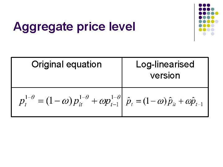
Aggregate price level Original equation Log-linearised version

Optimal price setting Original equation Log-linearised version

Myopic price Original equation Log-linearised version

Marginal cost Original equation Log-linearised version

Wages Original equation Log-linearised version

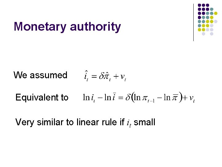
Monetary authority We assumed Equivalent to Very similar to linear rule if it small

Log-linearised DSGE model Monetary authority Firms Households

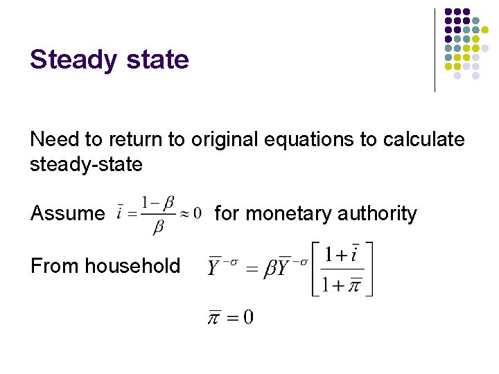
Steady state Need to return to original equations to calculate steady-state Assume From household for monetary authority

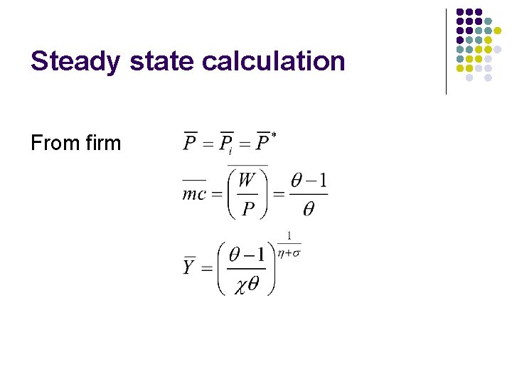
Steady state calculation From firm

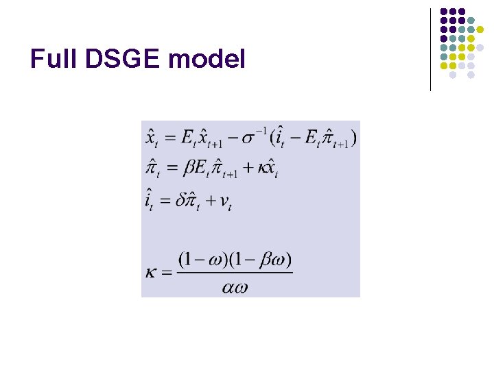
Full DSGE model

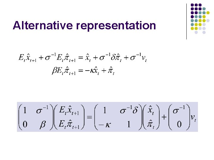
Alternative representation

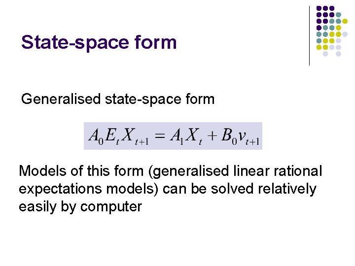
State-space form Generalised state-space form Models of this form (generalised linear rational expectations models) can be solved relatively easily by computer

Next steps Derive a solution for log-linearised models Blanchard-Kahn technique