Statistical model of quiet Sun coronal heating Elena

Statistical model of quiet Sun coronal heating Elena Podladchikova LPCE/CNRS, France Max-Planck-Institut für Aeronomie 1

Ø Introduction – The heating problem – Generalities about the solar corona – Heating mechanisms: • waves • DC currents – Eruptions and power-laws. Problem of the scales – Statistical models built on Self-Organized Criticality (SOC) 2

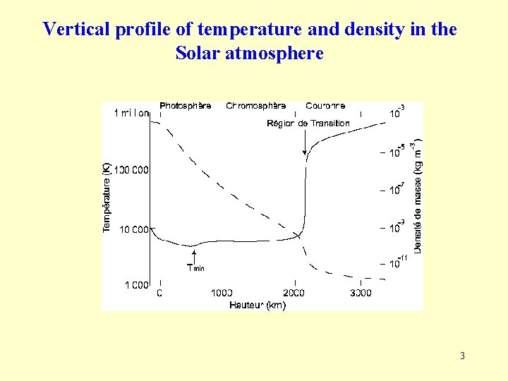
Vertical profile of temperature and density in the Solar atmosphere 3

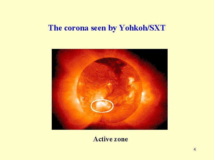
The corona seen by Yohkoh/SXT Active zone 4

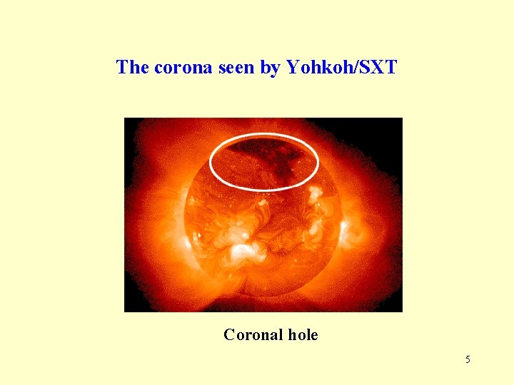
The corona seen by Yohkoh/SXT Coronal hole 5

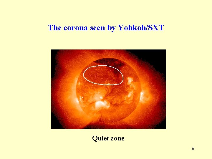
The corona seen by Yohkoh/SXT Quiet zone 6

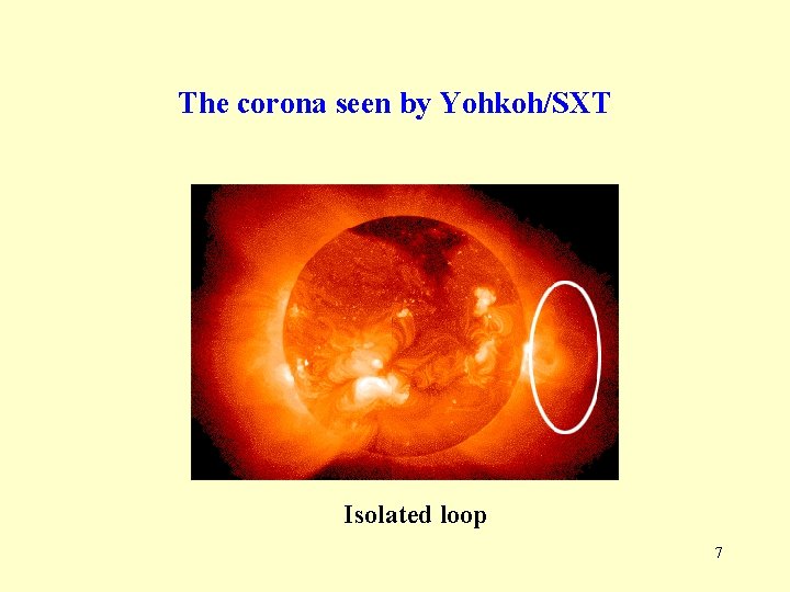
The corona seen by Yohkoh/SXT Isolated loop 7

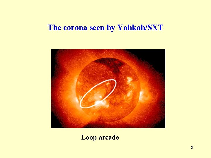
The corona seen by Yohkoh/SXT Loop arcade 8

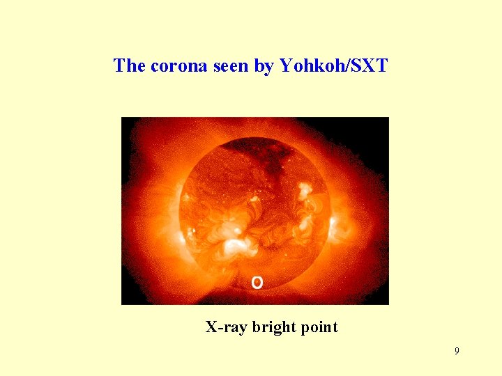
The corona seen by Yohkoh/SXT X-ray bright point 9

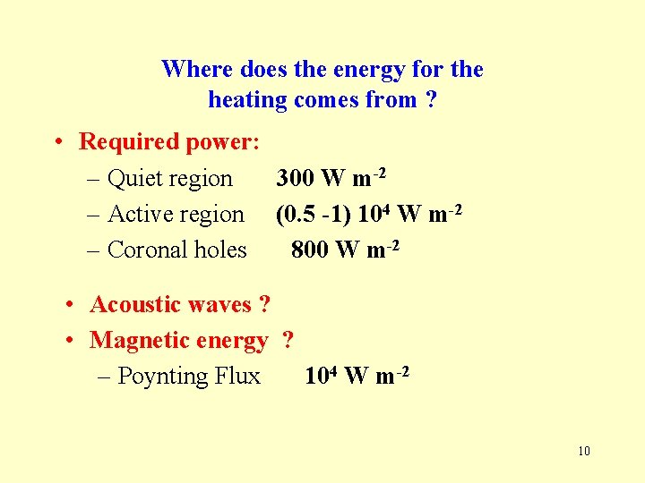
Where does the energy for the heating comes from ? • Required power: – Quiet region 300 W m-2 – Active region (0. 5 -1) 104 W m-2 – Coronal holes 800 W m-2 • Acoustic waves ? • Magnetic energy ? – Poynting Flux 104 W m-2 10

Dissipation of magnetic energy Ø Heating by MHD waves – – – Dissipation of Alfvén waves (Alfvén 1947) Resonance absorption (Ionson 1978) Phase mixing (Heyvaerts & Priest 1983) Ion cyclotron waves (Mc. Kenzie et al. 1995) Turbulence Ø Heating by dissipation of DC – Anomalous resistivity or double layers – Reconnection (Giovanelli 1946) – Anomalous resistivity or double layers 11

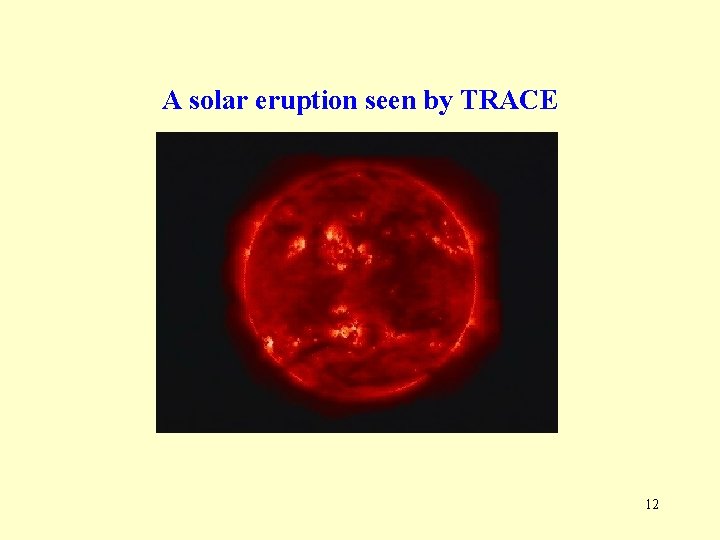
A solar eruption seen by TRACE 12

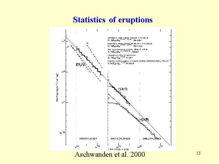
Statistics of eruptions Aschwanden et al. 2000 13

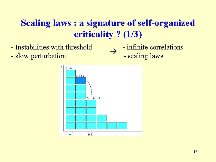
Scaling laws : a signature of self-organized criticality ? (1/3) - Instabilities with threshold - slow perturbation - infinite correlations - scaling laws 14

Statistical models are appropriate: • No inertial interval • Small scale events – only statistical information • Scales problems: V (Energy accumulation) >> V (Energy dissipation) • Heating occurs not due to a single event but depends on the frequency of events, the spatial distribution, etc. . . • CA can simulate large number of dissipative events and their statistics. • Statistical models allow to make a phenomenological description with different physical effects which can be easily considered in these models but with difficulty in MHD. 15

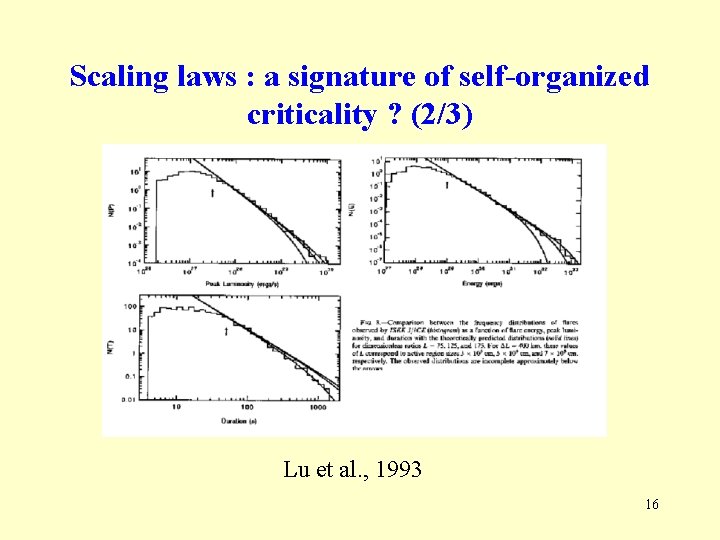
Scaling laws : a signature of self-organized criticality ? (2/3) Lu et al. , 1993 16

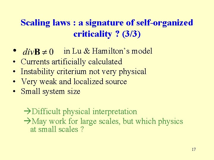
Scaling laws : a signature of self-organized criticality ? (3/3) • • • in Lu & Hamilton’s model Currents artificially calculated Instability criterium not very physical Very weak and localized source Small system size Difficult physical interpretation May work for large scales, but which physics at small scales ? 17

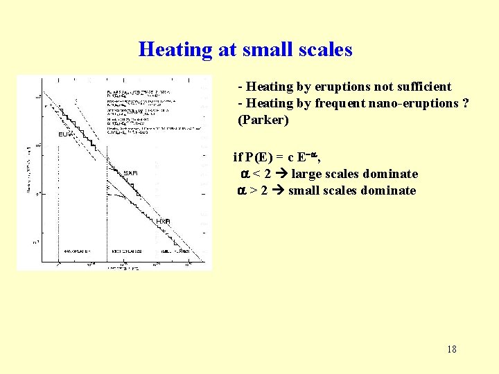
Heating at small scales - Heating by eruptions not sufficient - Heating by frequent nano-eruptions ? (Parker) if P(E) = c E-a, a < 2 large scales dominate a > 2 small scales dominate 18

Second part Model description • Why small-scale sources ? • Description of homogeneous sources • Dissipation mechanisms and their physical meaning 19

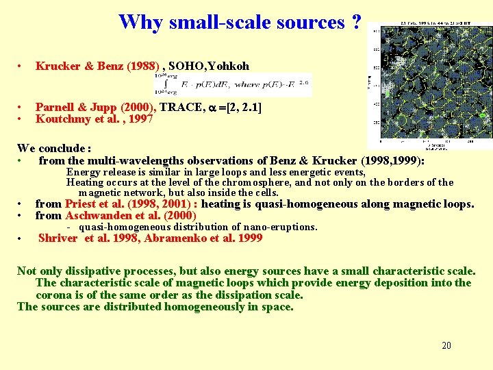
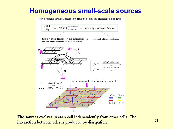
Why small-scale sources ? • Krucker & Benz (1988) , SOHO, Yohkoh • • Parnell & Jupp (2000), TRACE, a =[2, 2. 1] Koutchmy et al. , 1997 We conclude : • from the multi-wavelengths observations of Benz & Krucker (1998, 1999): Energy release is similar in large loops and less energetic events, Heating occurs at the level of the chromosphere, and not only on the borders of the magnetic network, but also inside the cells. • • from Priest et al. (1998, 2001) : heating is quasi-homogeneous along magnetic loops. from Aschwanden et al. (2000) • Shriver et al. 1998, Abramenko et al. 1999 - quasi-homogeneous distribution of nano-eruptions. Not only dissipative processes, but also energy sources have a small characteristic scale. The characteristic scale of magnetic loops which provide energy deposition into the corona is of the same order as the dissipation scale. The sources are distributed homogeneously in space. 20

Homogeneous small-scale sources The sources evolves in each cell independently from other cells. The interaction between cells is produced by dissipation. 21

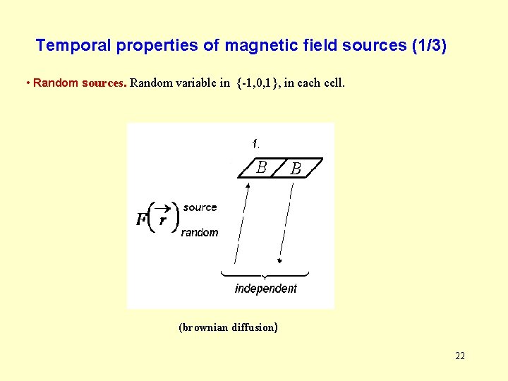
Temporal properties of magnetic field sources (1/3) • Random sources. Random variable in {-1, 0, 1}, in each cell. (brownian diffusion) 22

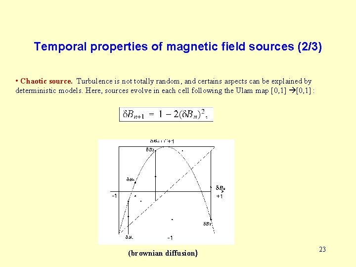
Temporal properties of magnetic field sources (2/3) • Chaotic source. Turbulence is not totally random, and certains aspects can be explained by deterministic models. Here, sources evolve in each cell following the Ulam map [0, 1] : (brownian diffusion) 23

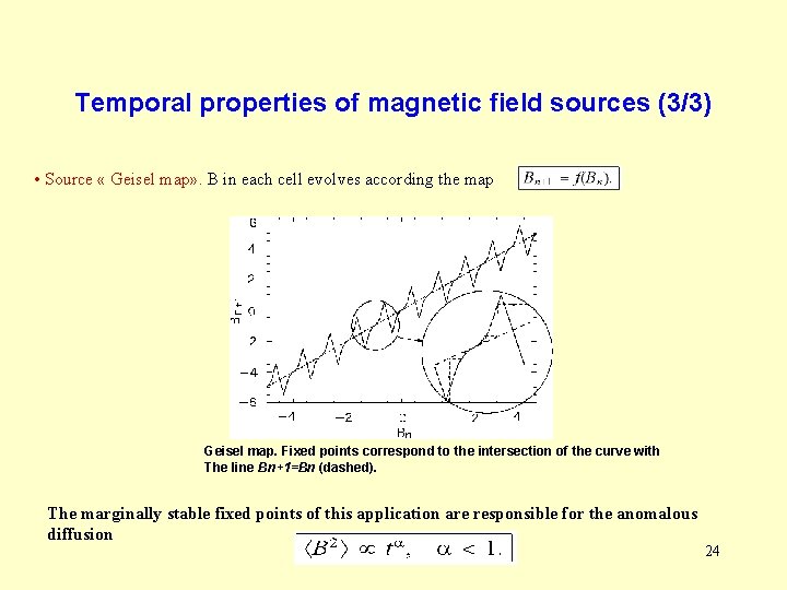
Temporal properties of magnetic field sources (3/3) • Source « Geisel map» . B in each cell evolves according the map Geisel map. Fixed points correspond to the intersection of the curve with The line Bn+1=Bn (dashed). The marginally stable fixed points of this application are responsible for the anomalous diffusion 24

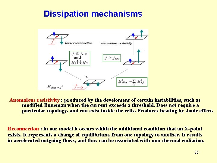
Dissipation mechanisms Anomalous resistivity : produced by the develoment of certain instabilities, such as modified Buneman when the current exceeds a threshold. Does not require a particular topology, and can exist inside the cells. Produces heating by Joule effect. Reconnection : in our model it occurs whith the additional condition that an X-point exists. It represents a change of equilibrium, from one topology to another. It results in accelerated outgoing flows, and thus can be associated with non-thermal radiation. 25

Third part How does the nature of dissipative phenomena influences the dissipated energy ? • Can local dissipative processes produce long-range spatial correlations ? • How does the spatial correlation length influences the statistics of dissipated energy ? 26

27

28

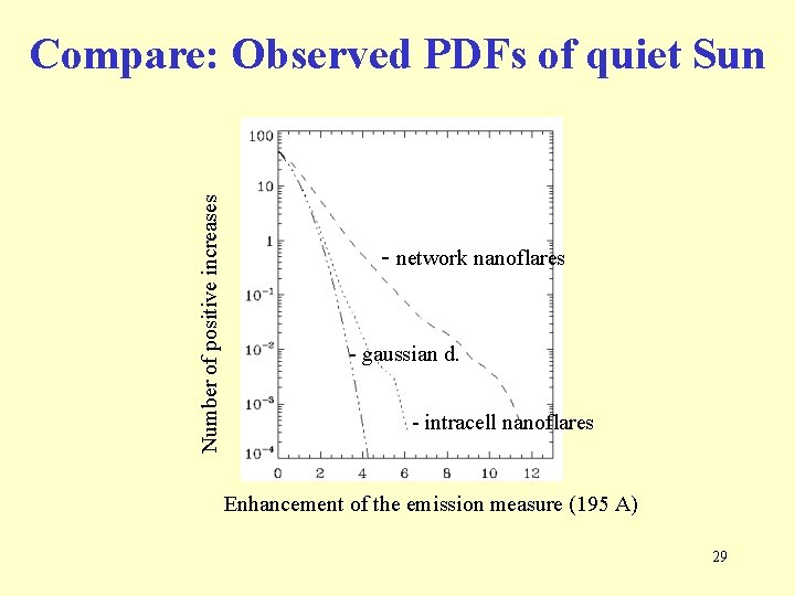
Number of positive increases Compare: Observed PDFs of quiet Sun - network nanoflares - gaussian d. - intracell nanoflares Enhancement of the emission measure (195 A) 29

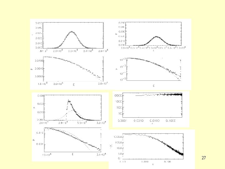
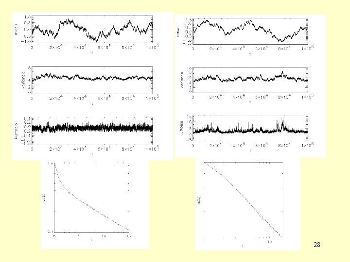
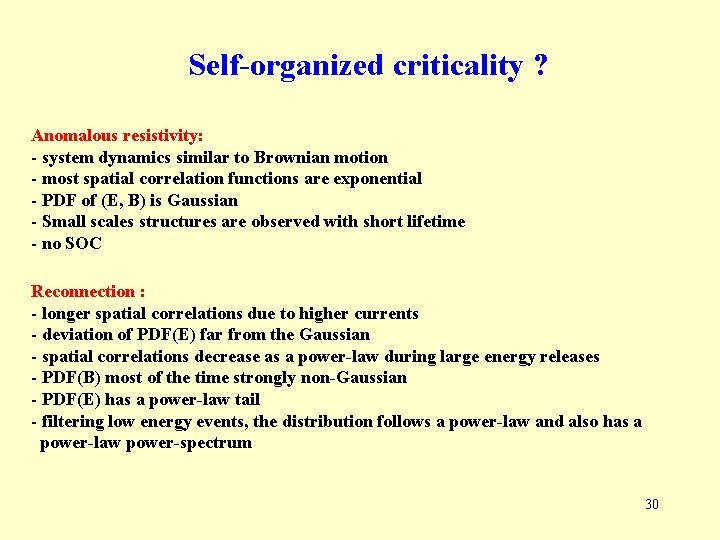
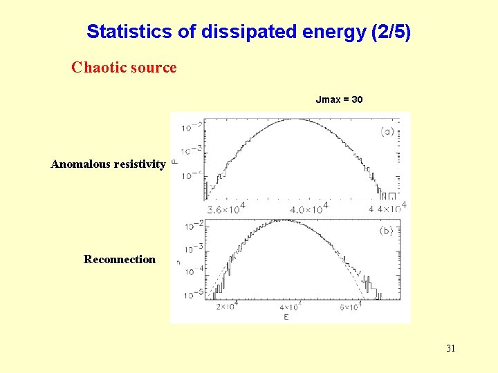
Self-organized criticality ? Anomalous resistivity: - system dynamics similar to Brownian motion - most spatial correlation functions are exponential - PDF of (E, B) is Gaussian - Small scales structures are observed with short lifetime - no SOC Reconnection : - longer spatial correlations due to higher currents - deviation of PDF(E) far from the Gaussian - spatial correlations decrease as a power-law during large energy releases - PDF(B) most of the time strongly non-Gaussian - PDF(E) has a power-law tail - filtering low energy events, the distribution follows a power-law and also has a power-law power-spectrum 30

Statistics of dissipated energy (2/5) Chaotic source Jmax = 30 Anomalous resistivity Reconnection 31

Statistics of dissipated energy (5/5) For large values of the threshold, we observe a suprathermal tail at high energies with a powerlaw shape. The absolute value of the exponent is bigger when dissipation is provided by reconnection rather than anomalous resistivity. This tendency is similar to the one found by Benz & Krucker (2000) who have studied augmentation of emission measures. 32

Fourth part Large scale magnetic structures driven by different sources 33

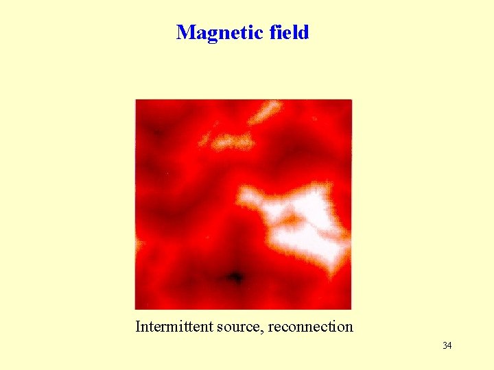
Magnetic field Intermittent source, reconnection 34

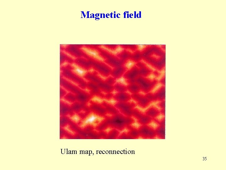
Magnetic field Ulam map, reconnection 35

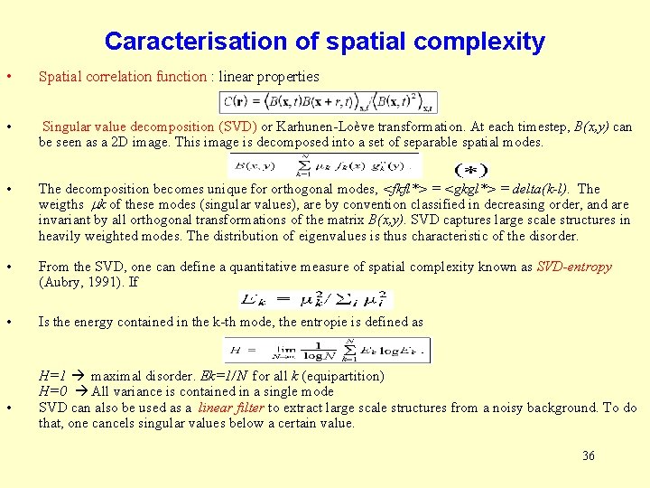
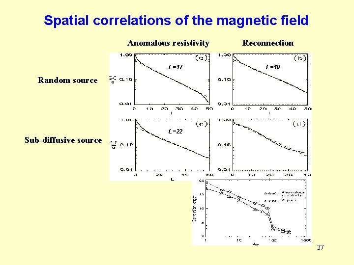
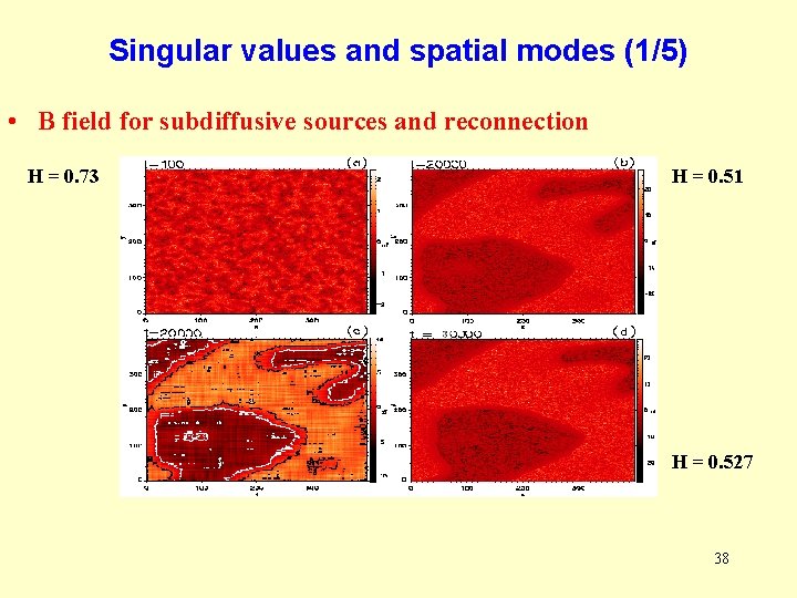
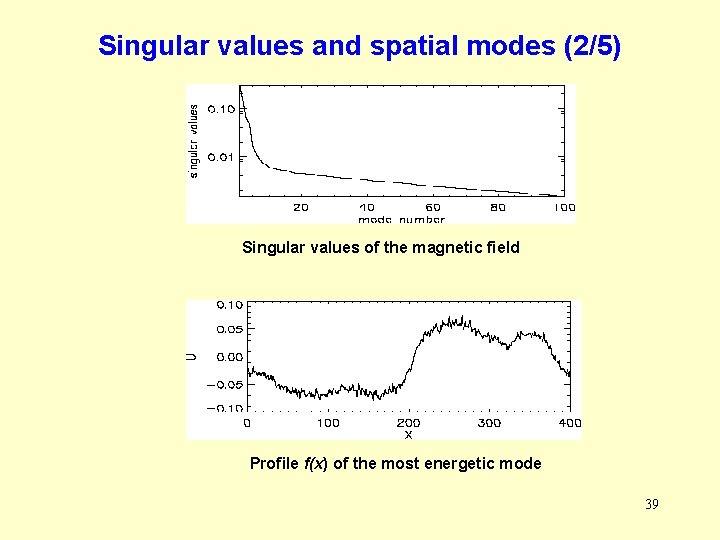
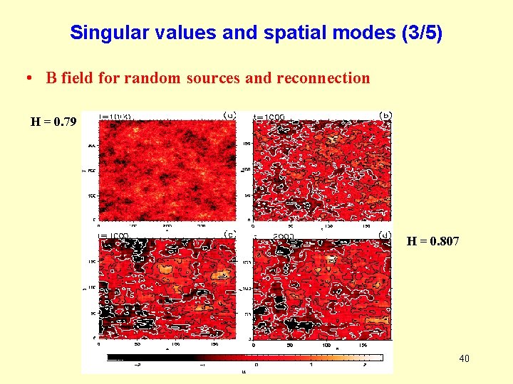
Caracterisation of spatial complexity • Spatial correlation function : linear properties • Singular value decomposition (SVD) or Karhunen-Loève transformation. At each timestep, B(x, y) can be seen as a 2 D image. This image is decomposed into a set of separable spatial modes. • The decomposition becomes unique for orthogonal modes, <fkfl*> = <gkgl*> = delta(k-l). The weigths k of these modes (singular values), are by convention classified in decreasing order, and are invariant by all orthogonal transformations of the matrix B(x, y). SVD captures large scale structures in heavily weighted modes. The distribution of eigenvalues is thus characteristic of the disorder. • From the SVD, one can define a quantitative measure of spatial complexity known as SVD-entropy (Aubry, 1991). If • Is the energy contained in the k-th mode, the entropie is defined as • H=1 maximal disorder. Ek=1/N for all k (equipartition) H=0 All variance is contained in a single mode SVD can also be used as a linear filter to extract large scale structures from a noisy background. To do that, one cancels singular values below a certain value. 36

Spatial correlations of the magnetic field Anomalous resistivity L=17 Reconnection L=19 Random source L=22 Sub-diffusive source 37

Singular values and spatial modes (1/5) • B field for subdiffusive sources and reconnection H = 0. 73 H = 0. 51 H = 0. 527 38

Singular values and spatial modes (2/5) Singular values of the magnetic field Profile f(x) of the most energetic mode 39

Singular values and spatial modes (3/5) • B field for random sources and reconnection H = 0. 79 H = 0. 807 40

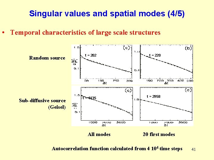
Singular values and spatial modes (4/5) • Temporal characteristics of large scale structures Random source t = 202 t = 220 Sub-diffusive source (Geisel) t = 1435 t = 2958 All modes 20 first modes Autocorrelation function calculated from 4 104 time steps 41

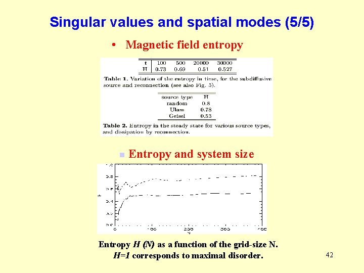
Singular values and spatial modes (5/5) • Magnetic field entropy n Entropy and system size Entropy H (N) as a function of the grid-size N. H=1 corresponds to maximal disorder. 42

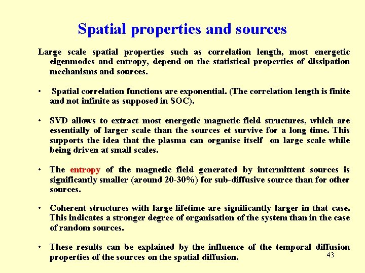
Spatial properties and sources Large scale spatial properties such as correlation length, most energetic eigenmodes and entropy, depend on the statistical properties of dissipation mechanisms and sources. • Spatial correlation functions are exponential. (The correlation length is finite and not infinite as supposed in SOC). • SVD allows to extract most energetic magnetic field structures, which are essentially of larger scale than the sources et survive for a long time. This supports the idea that the plasma can organise itself on large scale while being driven at small scales. • The entropy of the magnetic field generated by intermittent sources is significantly smaller (around 20 -30%) for sub-diffusive source than for other sources. • Coherent structures with large lifetime are significantly larger in that case. This indicates a stronger degree of organisation of the system than in the case of random sources. • These results can be explained by the influence of the temporal diffusion 43 properties of the sources on the spatial diffusion.

Classification of distributions by means of Pearson technique 44

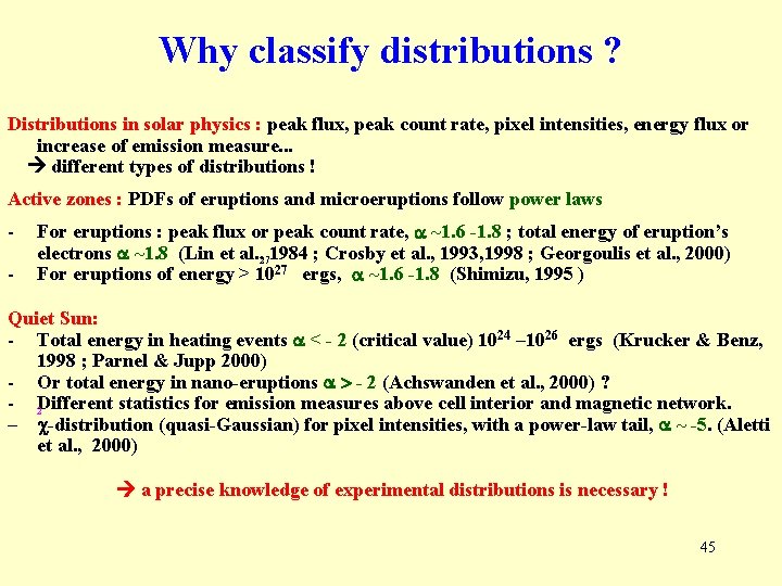
Why classify distributions ? Distributions in solar physics : peak flux, peak count rate, pixel intensities, energy flux or increase of emission measure. . . different types of distributions ! Active zones : PDFs of eruptions and microeruptions follow power laws - For eruptions : peak flux or peak count rate, a ~1. 6 -1. 8 ; total energy of eruption’s electrons a ~1. 8 (Lin et al. , 271984 ; Crosby et al. , 1993, 1998 ; Georgoulis et al. , 2000) For eruptions of energy > 1027 ergs, a ~1. 6 -1. 8 (Shimizu, 1995 ) Quiet Sun: - Total energy in heating events a < - 2 (critical value) 1024 – 1026 ergs (Krucker & Benz, 1998 ; Parnel & Jupp 2000) - Or total energy in nano-eruptions a > - 2 (Achswanden et al. , 2000) ? - 2 Different statistics for emission measures above cell interior and magnetic network. - c-distribution (quasi-Gaussian) for pixel intensities, with a power-law tail, a ~ -5. (Aletti et al. , 2000) a precise knowledge of experimental distributions is necessary ! 45

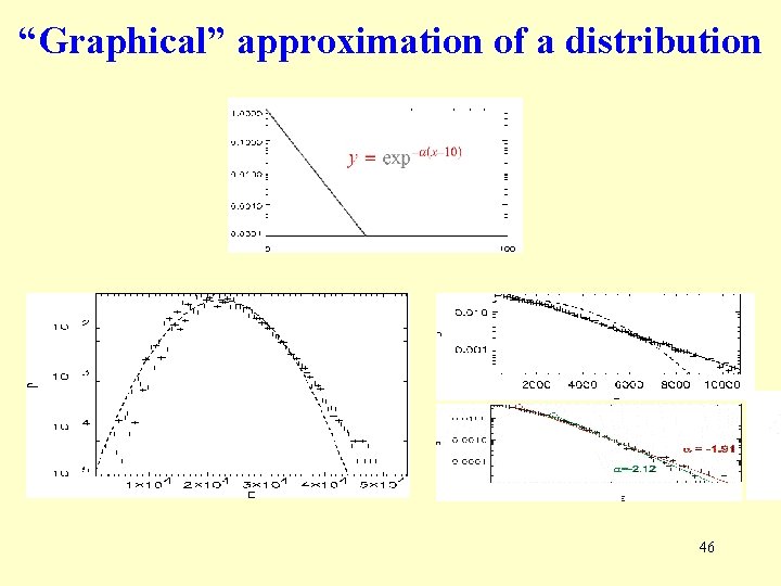
“Graphical” approximation of a distribution 46

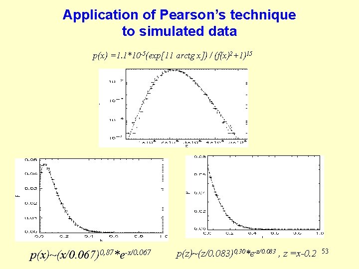
• An optimal approximation allows to : – Predict and compare theories and models – Classify distributions, for exemple to associate them with different physical phenomena • A study of empirical distributions and their fit by theoretical ones should fulfill the following conditions: – Objectivity – Automatisation – Results should be presented under a compact form • Pearson proposed a classification from : – Relationship between the first 4 moments – Fit by functions belonging to a large class of known distributions 47

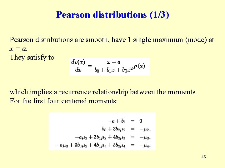
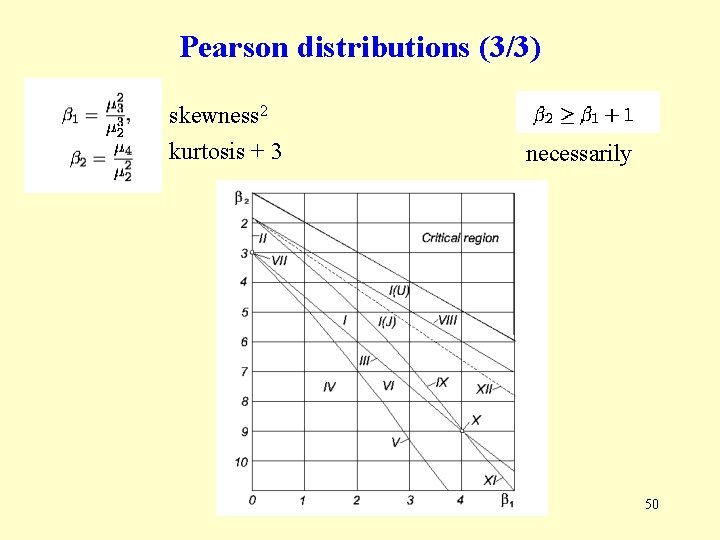
Pearson distributions (1/3) Pearson distributions are smooth, have 1 single maximum (mode) at x = a. They satisfy to which implies a recurrence relationship between the moments. For the first four centered moments: 48

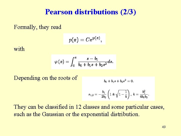
Pearson distributions (2/3) Formally, they read with Depending on the roots of They can be classified in 12 classes and some particular cases, such as the Gaussian or the exponential distribution. 49

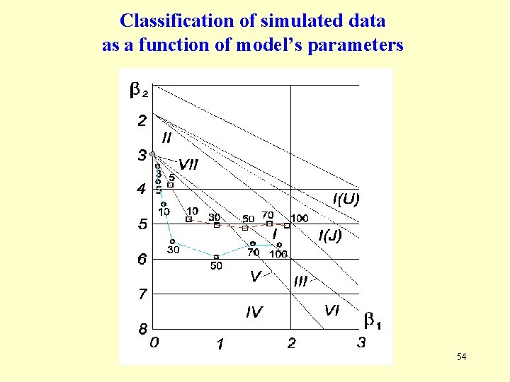
Pearson distributions (3/3) skewness 2 kurtosis + 3 necessarily 50

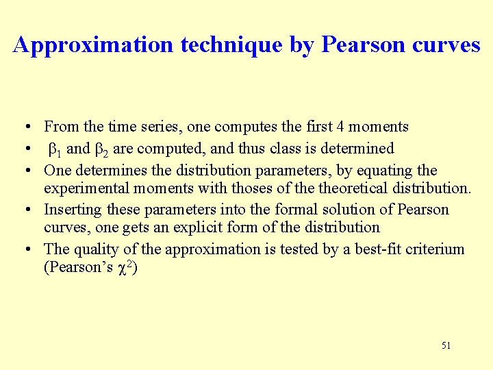
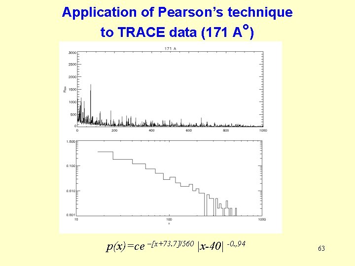
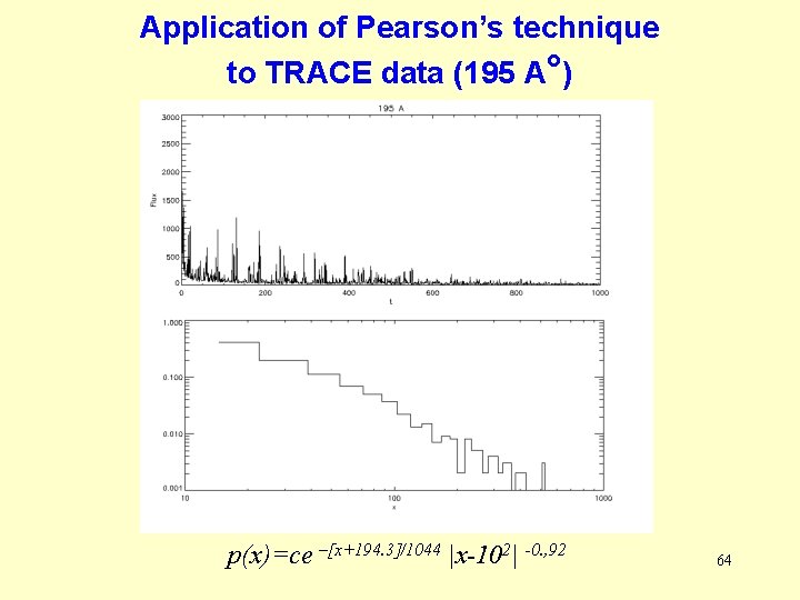
Approximation technique by Pearson curves • From the time series, one computes the first 4 moments • b 1 and b 2 are computed, and thus class is determined • One determines the distribution parameters, by equating the experimental moments with thoses of theoretical distribution. • Inserting these parameters into the formal solution of Pearson curves, one gets an explicit form of the distribution • The quality of the approximation is tested by a best-fit criterium (Pearson’s 2) 51

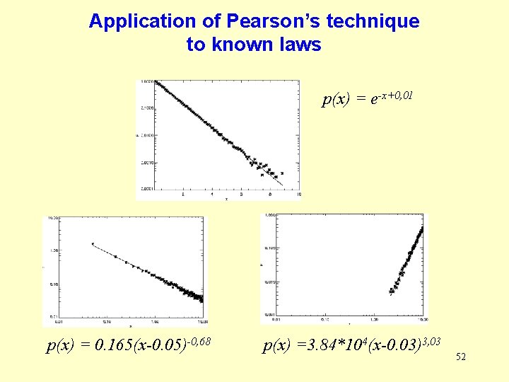
Application of Pearson’s technique to known laws p(x) = e-x+0, 01 p(x) = 0. 165(x-0. 05)-0, 68 p(x) =3. 84*104(x-0. 03)3, 03 52

Application of Pearson’s technique to simulated data p(x) =1. 1*10 -5(exp[11 arctg x]) / (f(x)2+1)15 p(x)~(x/0. 067)0, 87*e-x/0. 067 p(z)~(z/0. 083)0, 30*e-z/0. 083 , z =x-0. 2 53

Classification of simulated data as a function of model’s parameters 54

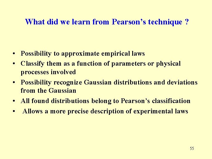
What did we learn from Pearson’s technique ? • Possibility to approximate empirical laws • Classify them as a function of parameters or physical processes involved • Possibility recognize Gaussian distributions and deviations from the Gaussian • All found distributions belong to Pearson’s classification • Allows a more precise description of experimental laws 55

Some perspectives 56

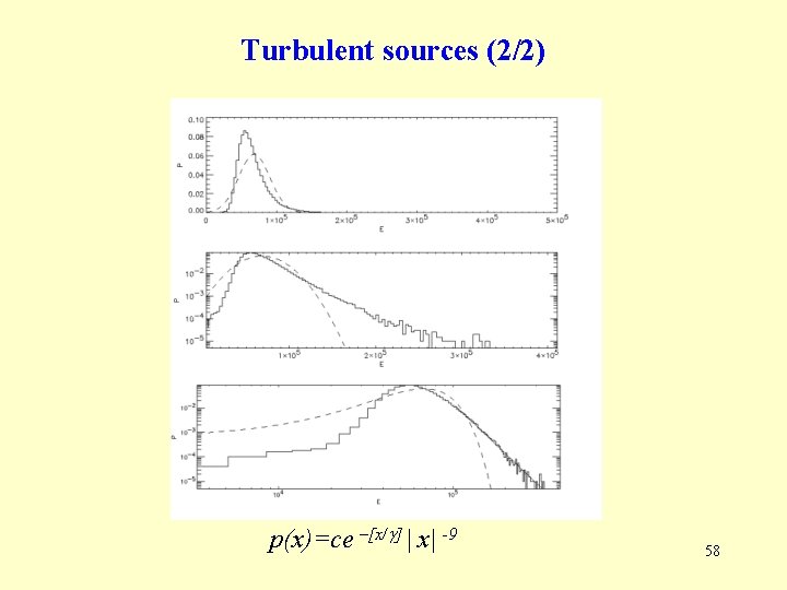
Turbulent sources (1/2) • Why ? - photospheric convection is partly turbulent, for example in between granules - a power-law spectrum allows to change the relative weights of differents scales. This allows to study the influence of the characteristic scales of the source. • How ? - power-law spectrum + random phases, independant, at each time step 57

Turbulent sources (2/2) p(x)=ce –[x/g] | x| -9 58

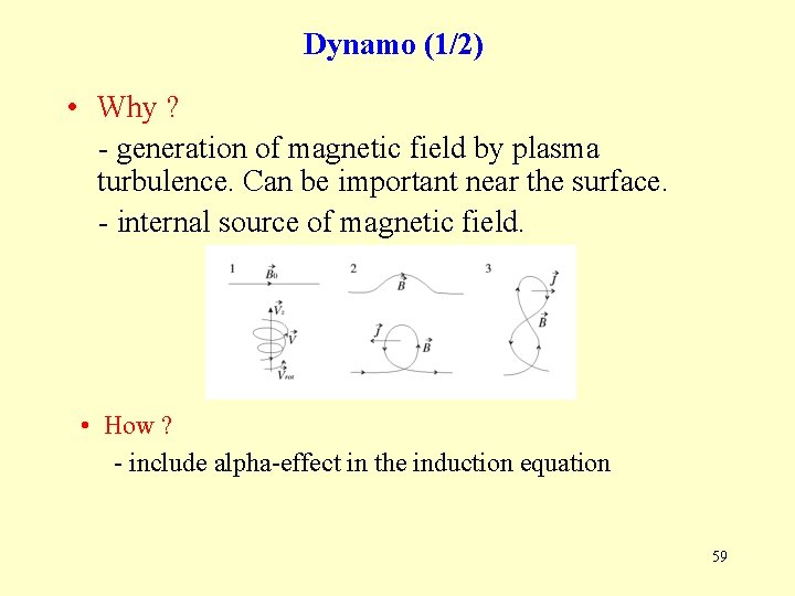
Dynamo (1/2) • Why ? - generation of magnetic field by plasma turbulence. Can be important near the surface. - internal source of magnetic field. • How ? - include alpha-effect in the induction equation 59

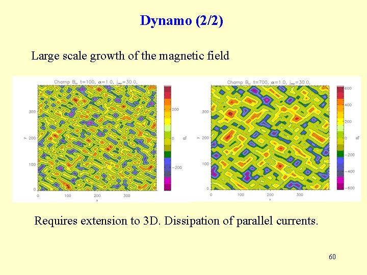
Dynamo (2/2) Large scale growth of the magnetic field Requires extension to 3 D. Dissipation of parallel currents. 60

Conclusion and perspectives Recent observations from satellites such as So. HO or TRACE, due to their high resolution, have made even more important the questions of the characteristic scales of the heating. We have examined a statistical model of heating at small scales. In this model, we have studied small scale sources and dissipative processes. Their influence on the statistical properties of the heating was studied in detail. 61

Conclusion and perspectives The model thus presents some properties qualitatively similar to certain observations. It is flexible enough to be improved and augmented by the addition of new effects: - Study of the role of characteristics scales of the sources, with « turbulent sources » - generation of B-field by dynamo effect - Improve and combine reconnection and anomalous resistivity - Separate energy transformed into heating and acceleration - Detailed validation with experimental data - Extension to 3 D - … 62

Application of Pearson’s technique to TRACE data (171 A°) p(x)=ce –[x+73. 7]/560 |x-40| -0. , 94 63

Application of Pearson’s technique to TRACE data (195 A°) p(x)=ce –[x+194. 3]/1044 |x-102| -0. , 92 64