Statistical Genomics Lecture 7 Imputation Zhiwu Zhang Washington

Statistical Genomics Lecture 7: Imputation Zhiwu Zhang Washington State University

Outline • Why imputation • Accuracy evaluation • Mechanism of imputation ØHaplotype ØStochastic imputation ØNearest neighbors • Two packages ØKNN ØBEAGLE

Why imputation • Most of analyses do not allow missing data • Increase marker density • Meta analyses for multiple studies • Improve GWAS and GS

Imputation improve density • • • Coverage: 1 X Missing rate: 38% Imputed by KNN Filling rate: 97% Accuracy: 98% 3 M SNPs remain Huang et al. 2010, Nature Genetics

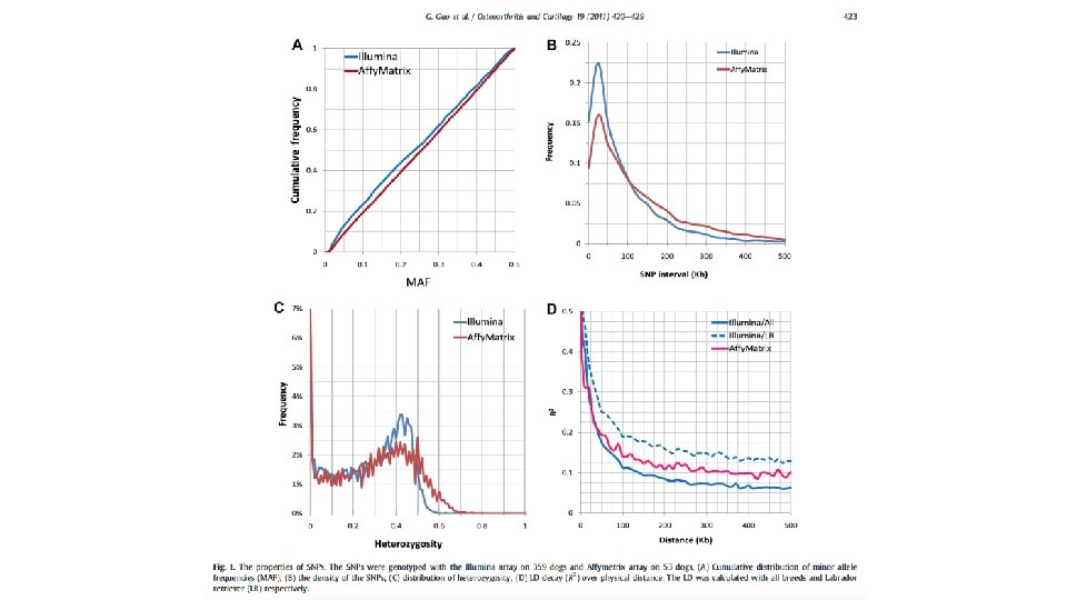
Example of meta analysis Guo et. al. Osteoarthritis Cartilage. 2011, 19(4): 420– 429 Fig. 5. Missing rate of SNPs. There were 21, 455 SNPs on Illumina array that was used to derive the predictive formula. Aboutw 40% of these SNPs were not present on the Affymetrix array that was used to genotype the dogs for independent validation (including the first and the third most influential SNPs on the Illumina array). The cumulative missing rates of SNPs are plotted against their order (descending log scale) based on their scaling factor.

Canine hip dysplasia is predictable

Imputation mechanism • Fill with mean • By major allele • Haplotype • Stochastic imputation with allele frequency • KNN • Hidden Marcov Model (BEAGLE) • Much more

Impute by haplotype Marchini et. al. Nat Rev Genet. 2010 Jul; 11(7): 499 -511

Stochastic imputation with allele frequency In case of inbred with alleles A or B, the frequency of A is f(A). If x has uniform distribution U(0, 1), then missing allele N can be imputed as

Implication of stochastic imputation #Define Stochastic Impute funciton Stochastic. Impute = function(X){ n=nrow(X) m=ncol(X) fn=col. Sums(X, na. rm=T) # sum of genotypes for all individuals fc=col. Sums(floor(X/3+1), na. rm=T) #count number of non missing individuals fa=fn/(2*fc) #Frequency of allele "2" for(i in 1: m){ index. a=runif(n)<fa[i] index. na=is. na(X[, i]) index. m 2=index. a & index. na index. m 0=!index. a & index. na X[index. m 2, i]=2 X[index. m 0, i]=0 } return(X)}

Evaluation of imputation accuracy • Randomly set a proportion of known data as missing • Impute the artificial missing • Compare the imputed and original

Import data #Import data my. GD=read. table(file="http: //zzlab. net/GAPIT/data/mdp_numeric. txt", head=T) X. raw=my. GD[, -1] #keep as original for comparison X=X. raw # Create a new variable than may be changed later

Variable of uniform distribution #Set missing values n=nrow(X) m=ncol(X) dp=m*n #total data points uv=runif(dp) hist(uv)

Missing value simulation mr=. 2 #missing rate missing=uv<mr length(missing) missing[1: 10] #Format indicator as matrix index. m=matrix(missing, n, m) dim(index. m) #Set missing values as NA X[index. m]=NA X. raw[1: 5, 1: 5] X[1: 5, 1: 5]

Two types of imputation accuracy • Correlation coefficient • Proportion of match

Accuracy calculation #Impute XI= Stochastic. Impute(X) #Correlation accuracy. r=cor(X. raw[index. m], XI[index. m]) #Proportion of match index. match=X. raw==XI index. mm=index. match&index. m accuracy. m=length(X[index. mm])/length(X[index. m]) accuracy. r accuracy. m

The two type accuracy are correlated nrep=100 myimp=replicate(nrep, { uv=runif(dp) #hist(uv) missing=uv<mr length(missing) missing[1: 10] index. m=matrix(missing, n, m) dim(index. m) X[index. m]=NA X. raw[1: 5, 1: 5] X[1: 5, 1: 5] #==================== #Impute with Stochastic. Impute XI= Stochastic. Impute(X) #Calcuate accuracy. r=cor(X. raw[index. m], XI[index. m]) index. match=X. raw==XI index. mm=index. match&index. m accuracy. m=length(X[index. mm])/length(X[index. m]) accuracy. r accuracy. m acc=c(accuracy. r, accuracy. m) }) plot(myimp[1, ], myimp[2, ])

Education Age US Election 2016

K Nearest Neighbors: vote Age • One neighbor: orange goes to blue • Five neighbors: orange goes to red Education

More dimension: Euclidean distance • Predict vote by education and age : n=2 • Impute missing genotypes: n is number of neighboring markers

"impute" R package #install. packages("impute") ## try http: // if https: // URLs are not supported source("https: //bioconductor. org/bioc. Lite. R") bioc. Lite("impute") library(impute) #Impute and calculate correlation XI= Stochastic. Impute(X) X. knn= impute. knn(as. matrix(t(X)), k=10) accuracy. r. si=cor(X. raw[index. m], XI[index. m]) accuracy. r. knn=cor(X. raw[index. m], t(X. knn$data)[index. m]) accuracy. r. si accuracy. r. knn

BEAGLE Brian Browning University of Washington Department of Medicine, Division of Medical Genetics Health Sciences Building, K-253 Box 357720 Seattle, WA 98195 -7720 Phone: (206) 685 -8482 Fax: (206) 543 -3050 E-mail: browning@uw. edu • Java package • JDK required • First release: 2006 • Current version: 5. 1 • Version used in class: 3. 3. 2 • Multiple papers https: //faculty. washington. edu/browning/beagle/b 3. html

Input file

Output file #Convert to BEAGLE input format index 0=X==0 index 1=X==1 index 2=X==2 indexna=is. na(X) X 2=X X 2[index 0]="At. A" X 2[index 1]="At. B" X 2[index 2]="Bt. B" X 2[indexna]="? t? " my. GD 2=cbind("M", my. GD[, 1], X 2) setwd("/Users/Zhiwu/Dropbox/Current/ZZLab/WSUCourse/CROPS 545/Demo") write. table(my. GD 2, file="test. bgl", quote=F, sep="t", col. name=F, row. name=F)

Run BEAGLE • Command line • From R #Impute with BEAGLE system("java -Xmx 12 g -jar /Users/Zhiwu/Dropbox/Current/ZZLab/WSUCourse/CROP S 545/Demo/Beagle/beagle. jar unphased=test. bgl missing=? out=test 1" )

Output of BEAGLE

Format conversion #Convert output format genotype. full <- read. delim("test 1. test. bgl. phased. gz", sep=" ", head=T) genotype. c=as. matrix(genotype. full[, -(1: 2)]) index. A=genotype. c=="A" index. B=genotype. c=="B" nr=nrow(genotype. c) nc=ncol(genotype. c) genotype. n=matrix(0, nr, nc) genotype. n[index. A]=0 genotype. n[index. B]=1 n 2=ncol(genotype. n) odd=seq(1, n 2 -1, 2) even=seq(2, n 2, 2) g 0=genotype. n[, odd] g 1=genotype. n[, even] X. bgl=g 0+g 1

Accuracy of BEAGLE #Impute and calculate correlation accuracy. r=cor(X. raw[index. m], X. bgl[index. m]) index. match=X. raw==X. bgl index. mm=index. match&index. m accuracy. m=length(X[index. mm])/length(X[index. m]) accuracy. r accuracy. m

Method comparison # Result comparison Method=c("Stochastic", "KNN", "BEAGLE") Cor=c(. 39, . 4, . 61) Match=c(. 33, . 65, . 75) par(mfrow=c(2, 1), mar = c(3, 4, 1, 1)) barplot(Cor, names. arg=Method, ylab="Correlation") barplot(Match, names. arg=Method, ylab="Match")

Highlight • Why imputation • How to impute • Stochastic imputation • KNN • BEAGLE • Accuracy evaluation