Statistical Genomics Lecture 15 MLM Zhiwu Zhang Washington

Objective From GLM to MLM Concept and working models Incorporating kinship for GWAS BLUE

GWAS by correlation my. GD=read. table(file="http: //zzlab. net/GAPIT/data/mdp_numeric. txt", head=T) my. GM=read. table(file="http: //zzlab.

color. vector <- rep(c("deepskyblue", "orange", "forestgreen", "indianred 3"), 10) m=nrow(my. GM) plot(t(-log 10(p))~seq(1: m),

QQ plot p. obs=p m 2=length(p. obs) p. uni=runif(m 2, 0, 1) order. obs=order(p.

Association with phenotypes r=-0. 32 PCA=prcomp(X) plot(my. Sim$y, PCA$x[, 2]) cor(my. Sim$y, PCA$x[, 2])

y=my. Sim$y G=my. GD[, -1] n=nrow(G) m=ncol(G) P=matrix(NA, 1, m) for (i in 1:

G=my. GD[, -1] n=nrow(G) m=ncol(G) P=matrix(NA, 1, m) for (i in 1: m){ x=G[,

More covariates observation mean b= [ b 0 y [1 PC 2 b 1

Recall for linear model y=b 0 + x 1 b 1 + x 2

Optimization to minimize residual =e'e =e 2=(y-Xb)2 ∂ /∂b =2 X'(y-Xb) =2 X'y-2 X'Xb=0

GLM (Conceptual) Phenotype on individuals Population structure y = SNP + Q (or PCs)

Minimize residual does not work for adding individuals' effects More parameters than observations Residuals

New rules Free individuals effects Only regulate the features for the population where they

MLM for GWAS Phenotype Population structure Unequal relatedness Y = SNP + Q (or

Fixed vs. Random Effects Fixed effect ü Limited levels ü Interest on levels Radom

Variance in MLM y = Xb + Zu + e Var(y)=V=Var(u)+Var(e) u prediction: Best

GWAS with MLM in GAPIT my. GAPIT=GAPIT( Y=my. Y, GD=my. GD, GM=my. GM, QTN.

GWAS by MLM library('MASS') # required for ginv library(multtest) library(gplots) library(compiler) #required for cmpfun

GWAS by GLM library('MASS') # required for ginv library(multtest) library(gplots) library(compiler) #required for cmpfun

Highlight From GLM to MLM Concept and working models Incorporating kinship for GWAS BLUE

Slides: 26

Download presentation

Statistical Genomics Lecture 15: MLM Zhiwu Zhang Washington State University

Objective From GLM to MLM Concept and working models Incorporating kinship for GWAS BLUE and BLUP MLM in GAPIT GLM in GAPIT

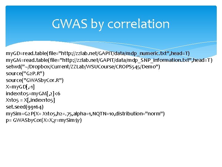
GWAS by correlation my. GD=read. table(file="http: //zzlab. net/GAPIT/data/mdp_numeric. txt", head=T) my. GM=read. table(file="http: //zzlab. net/GAPIT/data/mdp_SNP_information. txt", head=T) setwd("~/Dropbox/Current/ZZLab/WSUCourse/CROPS 545/Demo") source("G 2 P. R") source("GWASby. Cor. R") X=my. GD[, -1] index 1 to 5=my. GM[, 2]<6 X 1 to 5 = X[, index 1 to 5] set. seed(99164) my. Sim=G 2 P(X= X 1 to 5, h 2=. 75, alpha=1, NQTN=10, distribution="norm") p= GWASby. Cor(X=X, y=my. Sim$y)

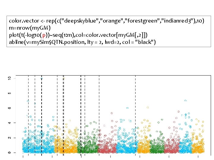
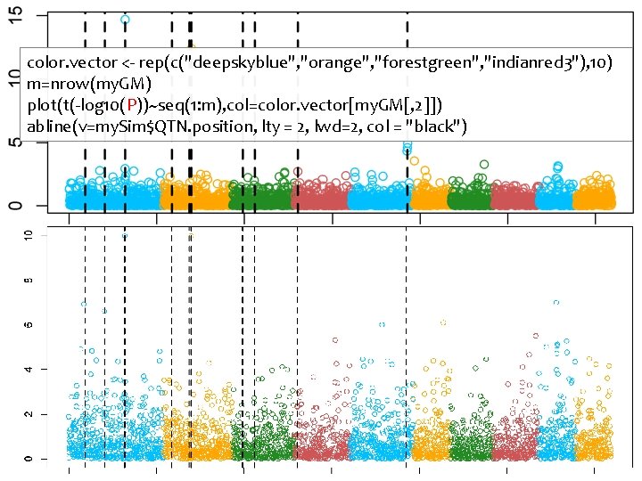
color. vector <- rep(c("deepskyblue", "orange", "forestgreen", "indianred 3"), 10) m=nrow(my. GM) plot(t(-log 10(p))~seq(1: m), col=color. vector[my. GM[, 2]]) abline(v=my. Sim$QTN. position, lty = 2, lwd=2, col = "black")

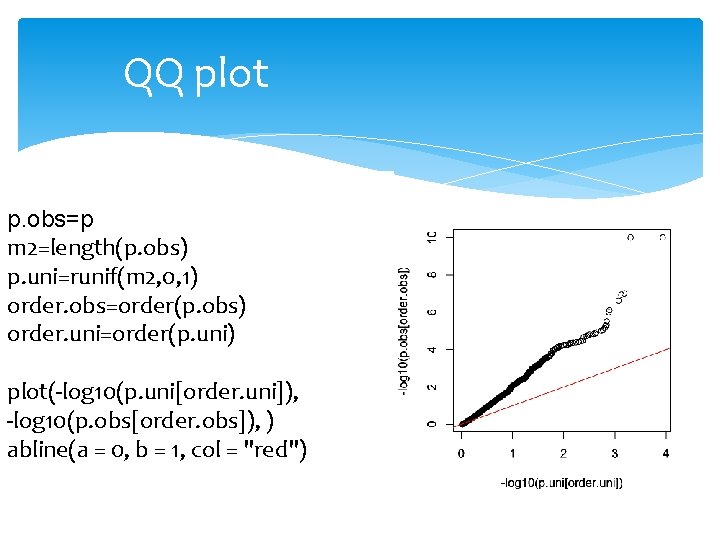
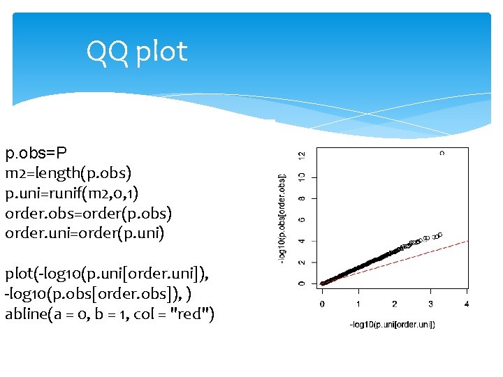
QQ plot p. obs=p m 2=length(p. obs) p. uni=runif(m 2, 0, 1) order. obs=order(p. obs) order. uni=order(p. uni) plot(-log 10(p. uni[order. uni]), -log 10(p. obs[order. obs]), ) abline(a = 0, b = 1, col = "red")

Association with phenotypes r=-0. 32 PCA=prcomp(X) plot(my. Sim$y, PCA$x[, 2]) cor(my. Sim$y, PCA$x[, 2])

y=my. Sim$y G=my. GD[, -1] n=nrow(G) m=ncol(G) P=matrix(NA, 1, m) for (i in 1: m){ x=G[, i] if(max(x)==min(x)){ p=1}else{ X=cbind(1, PCA$x[, 2], x) Add 2 nd PC as covariate LHS=t(X)%*%X C=solve(LHS) RHS=t(X)%*%y b=C%*%RHS yb=X%*%b e=y-yb n=length(y) ve=sum(e^2)/(n-1) vt=C*ve t=b/sqrt(diag(vt)) p=2*(1 -pt(abs(t), n-2)) } #end of testing variation P[i]=p[length(p)] } #end of looping for markers

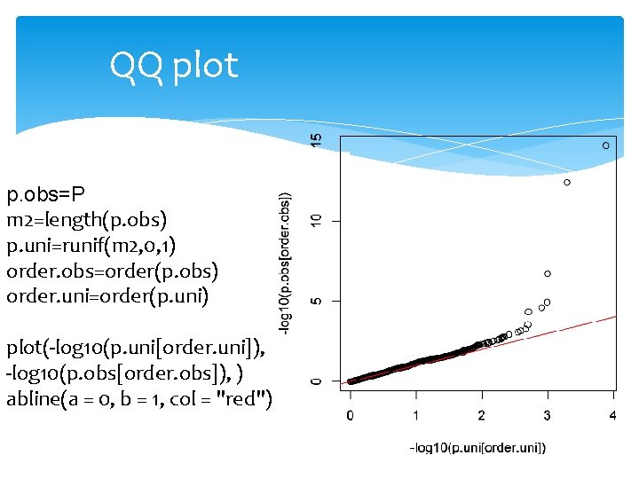
QQ plot p. obs=P m 2=length(p. obs) p. uni=runif(m 2, 0, 1) order. obs=order(p. obs) order. uni=order(p. uni) plot(-log 10(p. uni[order. uni]), -log 10(p. obs[order. obs]), ) abline(a = 0, b = 1, col = "red")

G=my. GD[, -1] n=nrow(G) m=ncol(G) P=matrix(NA, 1, m) for (i in 1: m){ x=G[, i] if(max(x)==min(x)){ p=1}else{ X=cbind(1, PCA$x[, 1: 3], x) LHS=t(X)%*%X C=solve(LHS) RHS=t(X)%*%y b=C%*%RHS yb=X%*%b e=y-yb n=length(y) ve=sum(e^2)/(n-1) vt=C*ve t=b/sqrt(diag(vt)) p=2*(1 -pt(abs(t), n-2)) } #end of testing variation P[i]=p[length(p)] } #end of looping for markers Using more PCs

color. vector <- rep(c("deepskyblue", "orange", "forestgreen", "indianred 3"), 10) m=nrow(my. GM) plot(t(-log 10(P))~seq(1: m), col=color. vector[my. GM[, 2]]) abline(v=my. Sim$QTN. position, lty = 2, lwd=2, col = "black")

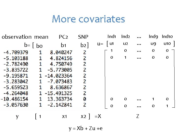
More covariates observation mean b= [ b 0 y [1 PC 2 b 1 x 1 SNP b 2 ] u= x 2 ] =X y = Xb + Zu +e Ind 1 [ u 1 1 0 Ind 2 u 2 0 1 … … 0 0 … … Z Ind 9 Ind 10 u 9 u 10 ] 0 0 1

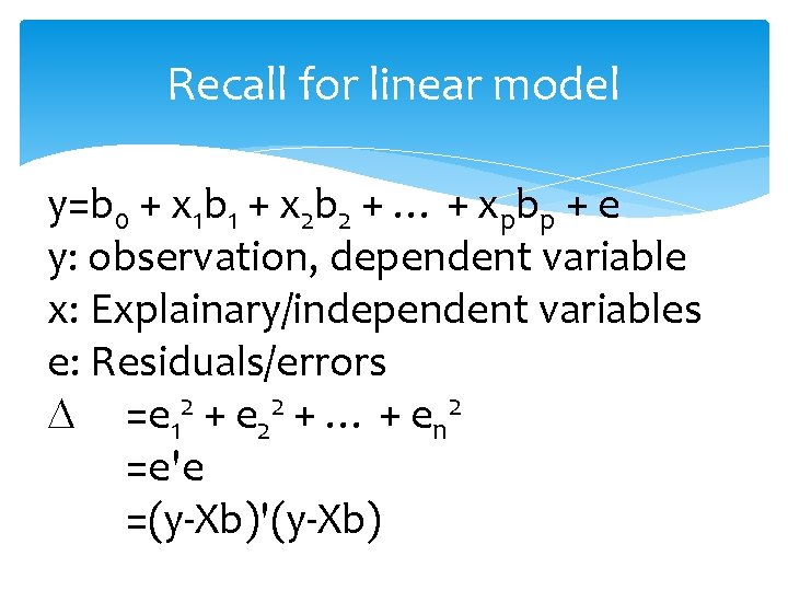
Recall for linear model y=b 0 + x 1 b 1 + x 2 b 2 + … + xpbp + e y: observation, dependent variable x: Explainary/independent variables e: Residuals/errors =e 12 + e 22 + … + en 2 =e'e =(y-Xb)'(y-Xb)

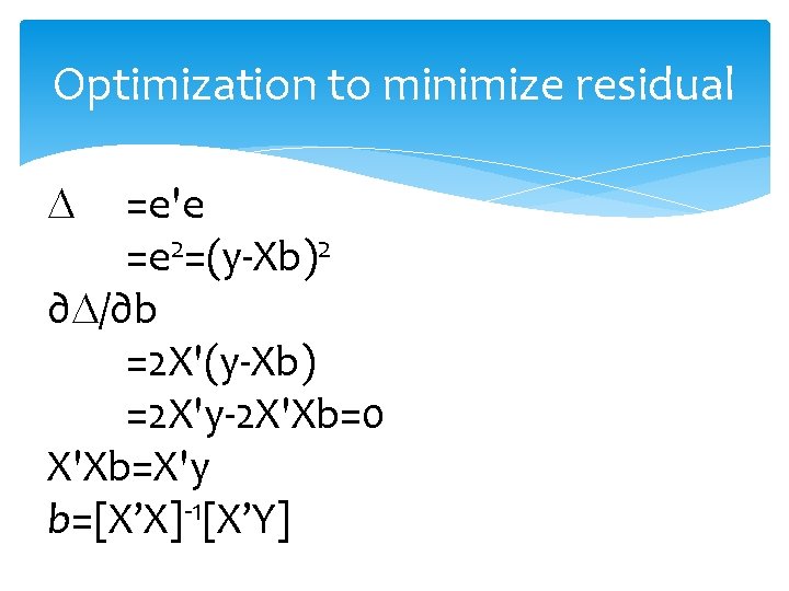
Optimization to minimize residual =e'e =e 2=(y-Xb)2 ∂ /∂b =2 X'(y-Xb) =2 X'y-2 X'Xb=0 X'Xb=X'y b=[X’X]-1[X’Y]

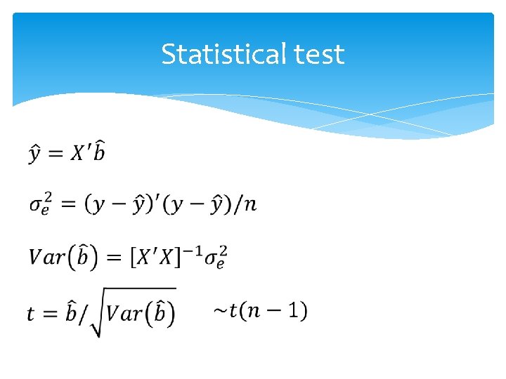
Statistical test

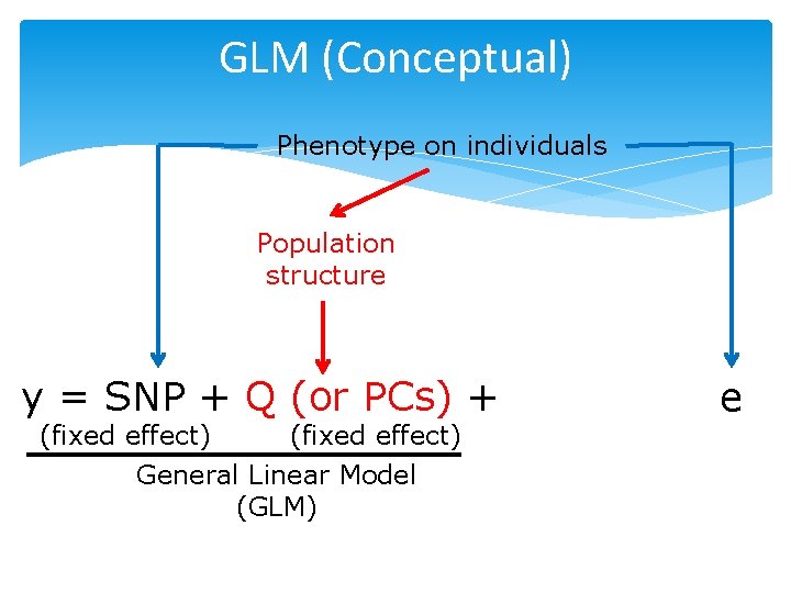
GLM (Conceptual) Phenotype on individuals Population structure y = SNP + Q (or PCs) + (fixed effect) General Linear Model (GLM) e

Minimize residual does not work for adding individuals' effects More parameters than observations Residuals are always zero due to over model fitting Needs new rules

New rules Free individuals effects Only regulate the features for the population where they from: means (0) and variances Optimize variances according to kinship and observation to maximize the likelihood

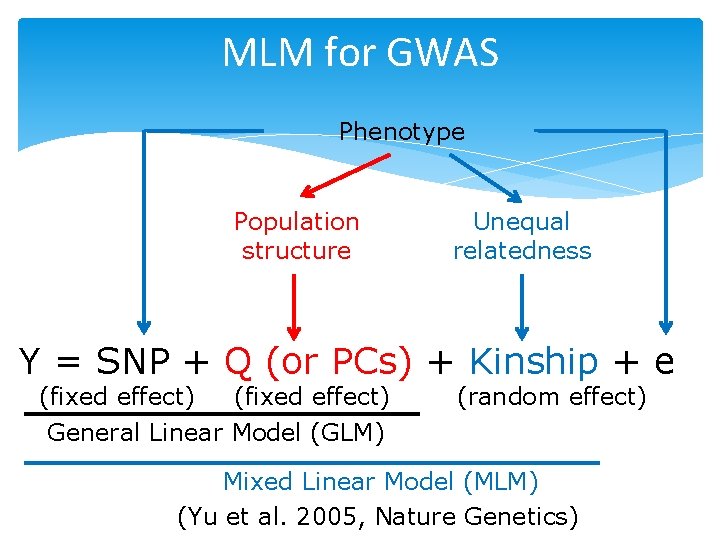
MLM for GWAS Phenotype Population structure Unequal relatedness Y = SNP + Q (or PCs) + Kinship + e (fixed effect) General Linear Model (GLM) (random effect) Mixed Linear Model (MLM) (Yu et al. 2005, Nature Genetics)

Fixed vs. Random Effects Fixed effect ü Limited levels ü Interest on levels Radom effect ü Many levels ü Interest on population behind the levels (mean, variance)

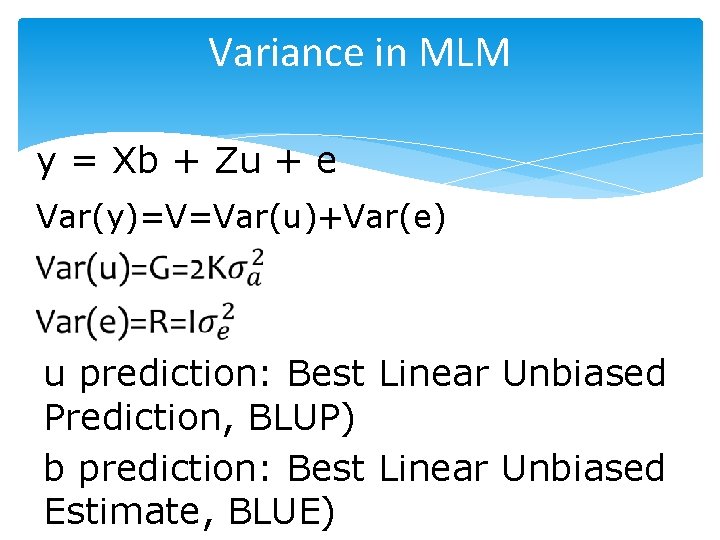
Variance in MLM y = Xb + Zu + e Var(y)=V=Var(u)+Var(e) u prediction: Best Linear Unbiased Prediction, BLUP) b prediction: Best Linear Unbiased Estimate, BLUE)

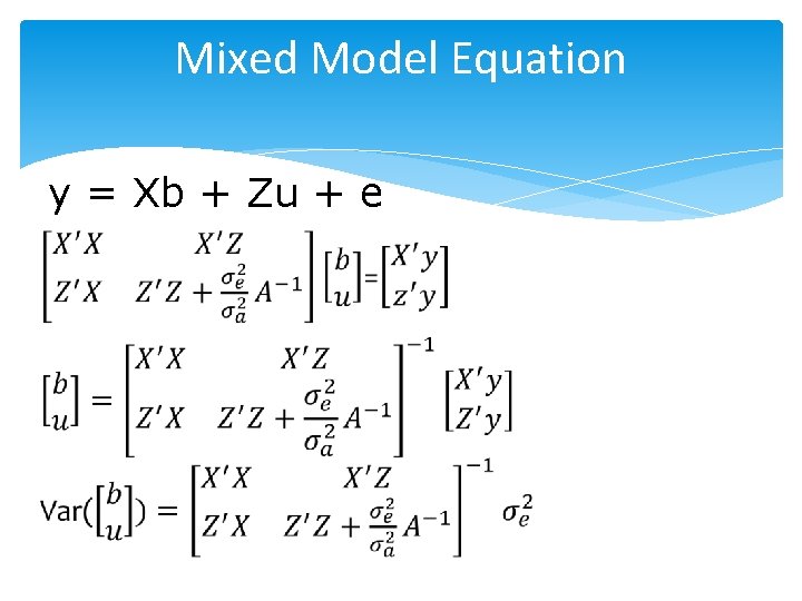
Mixed Model Equation y = Xb + Zu + e

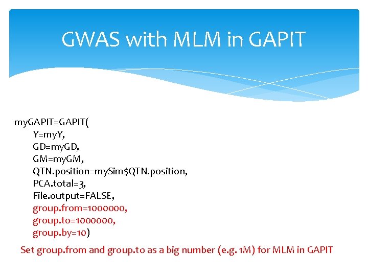
GWAS with MLM in GAPIT my. GAPIT=GAPIT( Y=my. Y, GD=my. GD, GM=my. GM, QTN. position=my. Sim$QTN. position, PCA. total=3, File. output=FALSE, group. from=1000000, group. to=1000000, group. by=10) Set group. from and group. to as a big number (e. g. 1 M) for MLM in GAPIT

GWAS by MLM library('MASS') # required for ginv library(multtest) library(gplots) library(compiler) #required for cmpfun library("scatterplot 3 d") source("http: //www. zzlab. net/GAPIT/emma. txt") source("http: //www. zzlab. net/GAPIT/gapit_functi ons. txt") my. GD=read. table(file="http: //zzlab. net/GAPIT/dat a/mdp_numeric. txt", head=T) my. GM=read. table(file="http: //zzlab. net/GAPIT/dat a/mdp_SNP_information. txt", head=T) setwd("~/Dropbox/Current/ZZLab/WSUCourse/CR OPS 545/Demo") source("G 2 P. R") set. seed(99164) my. Sim=G 2 P(X= X 1 to 5, h 2=. 75, alpha=1, NQTN=10, distribution="nor m") setwd("~/Desktop/temp") my. Y=cbind(as. data. frame(my. GD[, 1]), my. Sim$y) my. GAPIT=GAPIT( Y=my. Y, GD=my. GD, GM=my. GM, QTN. position=my. Sim$QTN. position, PCA. total=3, group. from=1000000, group. to=1000000, group. by=10, memo="MLM", file. output=TRUE, )

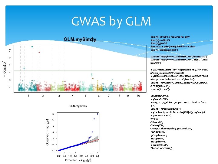
GWAS by GLM library('MASS') # required for ginv library(multtest) library(gplots) library(compiler) #required for cmpfun library("scatterplot 3 d") source("http: //www. zzlab. net/GAPIT/emma. txt") source("http: //www. zzlab. net/GAPIT/gapit_functi ons. txt") my. GD=read. table(file="http: //zzlab. net/GAPIT/dat a/mdp_numeric. txt", head=T) my. GM=read. table(file="http: //zzlab. net/GAPIT/dat a/mdp_SNP_information. txt", head=T) setwd("~/Dropbox/Current/ZZLab/WSUCourse/CR OPS 545/Demo") source("G 2 P. R") set. seed(99164) my. Sim=G 2 P(X= X 1 to 5, h 2=. 75, alpha=1, NQTN=10, distribution="nor m") setwd("~/Desktop/temp") my. Y=cbind(as. data. frame(my. GD[, 1]), my. Sim$y) my. GAPIT=GAPIT( Y=my. Y, GD=my. GD, GM=my. GM, QTN. position=my. Sim$QTN. position, PCA. total=3, group. from=1, group. to=1, group. by=10, memo="GLM", file. output=TRUE, )

Highlight From GLM to MLM Concept and working models Incorporating kinship for GWAS BLUE and BLUP MLM in GAPIT GLM in GAPIT